Introduction

In this project, I implemented diffusion model training and inference, as well as creating interesting anagrams with pretrained diffusion models.

Part A: Sampling Pretrained Models

Gaining Access to DeepFloyd

As a first step, let’s start with sampling with the DeepFloyd model with their infrastructure. We set the seed to 180 for reproducibility, and run the sampling process for the three text propts, “a man wearing a hat,” “a rocket ship,” and “an oil painting of a snowy mountain village,” for two different num_inference_steps of 20 and 50. This sampling results are presented below:

a man wearing a hat

a rocket ship

an oil painting of a snowy mountain village

Stage one sampling results with 20 inference steps

a man wearing a hat

a rocket ship

an oil painting of a snowy mountain village

Stage one sampling results with 50 inference steps

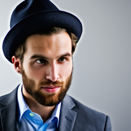
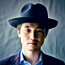
We can also upsample the images to 256x256 by passing them into the stage two encoder:

a man wearing a hat

a rocket ship

an oil painting of a snowy mountain village

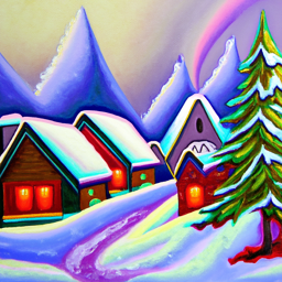
Stage two sampling results with 20 inference steps

a man wearing a hat

a rocket ship

an oil painting of a snowy mountain village

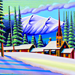
Stage two sampling results with 50 inference steps

We see that the qualities of the outputs are all good, even for the ones with fewer sampling steps. Furthermore, the content of the images matched well with the text prompt. This shows the incredible generation capability of diffusion models.

Implementing the Forward Process

We first implement the forward diffusion process. This process is given by the mathematical equation:

With the test image, we can test out three different noise levels [250, 500, 750]:

original

noise: 250

noise: 500

noise: 750

Campanile forward process

Classical Denoising

Using the fact that pixel-wise gaussian noise convolved with a gaussian kernel goes to zero as the kernel size increases (i.e. the expectation of gaussian noise is zero), we can remove the noise by applying a gaussian bluring in the price of hurting the images’ sharpness. Here, I use a gaussian kernel of size 9. This value is adjusted by empirically assess the output images quality.

original

blured noise 250

blured noise 500

blured noise 750

Classically denoised campanile

We see that gaussian bluring can remove some noise but the effectiveness quickly goes down as the noise level goes up.

One-Step Denoising

With a trained diffusion model, we can try denoising by subtracting off the estimated noise. Recall that:

By rearranging the terms and replace the gaussian noise with the model’s estimate \(\hat \epsilon_\theta(x_t)\), we get:

We can visualize the estimated denoised images:

original

one-step denoised 250

one-step denoised 500

one-step denoised 750

One-step denoised campanile

We see that the denoised images’ quality are much better than the classically denoised one. Moreover, while with low noise level the model is able to denoised to almost identical results, the one with higher noise levels have different details than the original image. This is due to the irreversible loss of information during the forward process.

Iterative Denoising

Instead of denoising with only one-shot estimate, we can denoise the image iteratively by applying the formula:

where \(v_{\sigma}(t, t')\) is a gaussian random variable with variance as a funciton of \(t\) and \(t'\), and \(\hat x_0\) is the one-shot estimate as in the section before. The idea is that we can try removing some noise from the image, then add some but less noise back into the image. This makes the denoising process stochastic and we can gain some stability by doing so. The process is visualized below. We start at t=690 (i_start=10).

0th iteration

5th iteration

10th iteration

15th iteration

20th iteration

22nd iteration (end)

Iteratively denoised campanile

We can compare different methods of denoising:

noised campanile

classically denoised

one-step denoised

iteratively denoised

Comparison of denoising methods

We see that classical method produce very low quality results. The one-step method is able to reconstruct a significant portion of the original image but missed out some details. The iteratively denoised one has a lot details but they are different from the original image! (it “fills in the blank”).

Diffusion Model Sampling

Instead of starting with a blurred image at some timestep, we can start at t=990 and feed in pure noise to sample with the model. Some results are showned below:

Some generated images

They look like image, but not so satisfactory.

Classifier-Free Guidance (CFG)

To improve the sampled images’ quality, we can use classifier free guidance. The idea is that given an “unconditional” prediction of noise and a “conditional” prediction of noise, we can manually go “more conditioned” by deviating from the unconditional prediction more. Mathematically, it can be written as:

where \(\epsilon_u\) is the unconditional prediction and the \(\epsilon_c\) is the conditional prediction. We use “” as the unconditional prompt and “a high quality photo” for unconditional prompt. The \(\gamma\) is chosen to be 7. Some samlping results are shown below:

Some images generated with CFG

Now the sampling results look a lot more like real photos.

Image-to-image Translation

SDEdit

We can also feed in a partially corropted (noised) image and then denoise from it. With different level of noise added, the sampling result will gradually deviate from the original image. We can exploit this fact to produce some interesting edit of the original image. Here, we test it out with three images:

original campanile

original oski

original tree

Original images

campanile from i=1

campanile from i=3

campanile from i=5

campanile from i=7

campanile from i=10

campanile from i=20

SDEdit campanile

Oski from i=1

Oski from i=3

Oski from i=5

Oski from i=7

Oski from i=10

Oski from i=20

SDEdit Oski

tree from i=1

tree from i=3

tree from i=5

tree from i=7

tree from i=10

tree from i=20

SDEdit tree

We can see that SDEdit was able to produce some interesting edits of the original images while retaining the rough structure of them. In particular, it worked well for campanile. However, for oski and tree, it does not work that well except for i=20. This could be due to the fact that during training time images like Oski and the tree was not seen that frequently and since diffusion model is a density modeling, it tends to drag all images to its training distribution conditioned on the text prompt. Therefore, Oski and the tree deviates from the original image a lot.

SDEdit with Unrealistic Images

original Gojo

original dog

original beach

Original images

Gojo from i=1

Gojo from i=3

Gojo from i=5

Gojo from i=7

Gojo from i=10

Gojo from i=20

SDEdit Gojo

dog from i=1

dog from i=3

dog from i=5

dog from i=7

dog from i=10

dog from i=20

SDEdit dog

beach from i=1

beach from i=3

beach from i=5

beach from i=7

beach from i=10

beach from i=20

SDEdit beach

We see that SDEdit works perfectly fine with unrealistic pictures. In particular, the beach image with only semantic coloring works the best. This is presumably due to the flexible yet informative conditioning that we provided to the model through the image.

Inpainting

We can also inpaint an image with a diffusion model. This is done by keeping the context along the “true” noising trajectory throughout the process. Namely, with a mask that is 0 for the context and 1 for the inpainting region, we iteratively do:

Here a few examples are presented:

original campanile

campanile mask

campanile to replace

inpainted campanile

Inpainted campanile

original Rick

Rick mask

Rick to replace

inpainted Rick

Inpainted Rick

original Pepe

Pepe mask

Pepe to replace

inpainted Pepe

Inpainted Pepe

With inpainting, we can create interesting edits of the original image wile keeping the context exactly the same as the original image. This allows us to do many cool things such as swapping out Rick’s head.

Text-Conditional Image-to-image Translation

Finally, we can condition the SDEdit algorithm on some text prompt. This is done by simply feeding in some text to the diffusion model denoiser. Here are three examples:

prompt: a rocket ship

prompt: a photo of a dog

prompt: a pencil

Original images and prompts

rocket ship from i=1

rocket ship from i=3

rocket ship from i=5

rocket ship from i=7

rocket ship from i=10

rocket ship from i=20

Text-conditioned rocket ship from campanile

dog from i=1

dog from i=3

dog from i=5

dog from i=7

dog from i=10

dog from i=20

Text-conditioned dog from Oski

tree from i=1

tree from i=3

tree from i=5

tree from i=7

tree from i=10

tree from i=20

Text-conditioned pencil from tree

Similar to the case before, campanile works the best while the latter two deviates from the original images a lot. Nevertheless, they are still conditioned well and successfully produced an edit that is controlled by the prompt.

Visual Anagrams

A very cool application of diffusion model is to use it to produce visual anagrams. To do so, we prepare two prompts. For the normal prompt we predict one estimate of noise. For the flipped prompt we predict one estimate based on the flipped image. The total estimate of noise is the average of the flipped estimates and the original estimates. This can be used in conjuction with CFG. Mathematically, it can we expressed as:

where \(\mathbf F\) is the flipping operator. I generated three examples of visual anagrams:

an oil painting of people around a campfire

a photo of a monkey

a photo of a wine glass

an oil painting of an old man

a photo of a programmer

a photo of a dress

Visual anagrams

The anagrams are quite impressive! This very simple method can produce high quality anagram is a great indication of the robustness of stochastic processes.

Hybrid Images

Finally, we can try to produce hybrid images. Similar to the idea of visual anagrams, we produce two sets of predictions with two prompts. They are passed through high and low pass filters respectively, and then sum together. When applying CFG, since these high and low pass filters combined becomes identity, we can simply do:

Some examples are:

low prompt: a lithograph of a skull
high prompt: a lithograph of waterfalls

low prompt: a picture of a concert
high prompt: a picture of sunset

low prompt: a photo of karaage
high prompt: a photo of poodles

Hybrid images

It does a reasonably good job on producing these hybrid images. However, we that karaage and poodles worked better than sunset and concert. This could be suggesting that we need closer prompts for this to work better.

Part B: Training a Diffusion Model from Scratch

Training a Single-Step Denoising UNet

Implementing the UNet

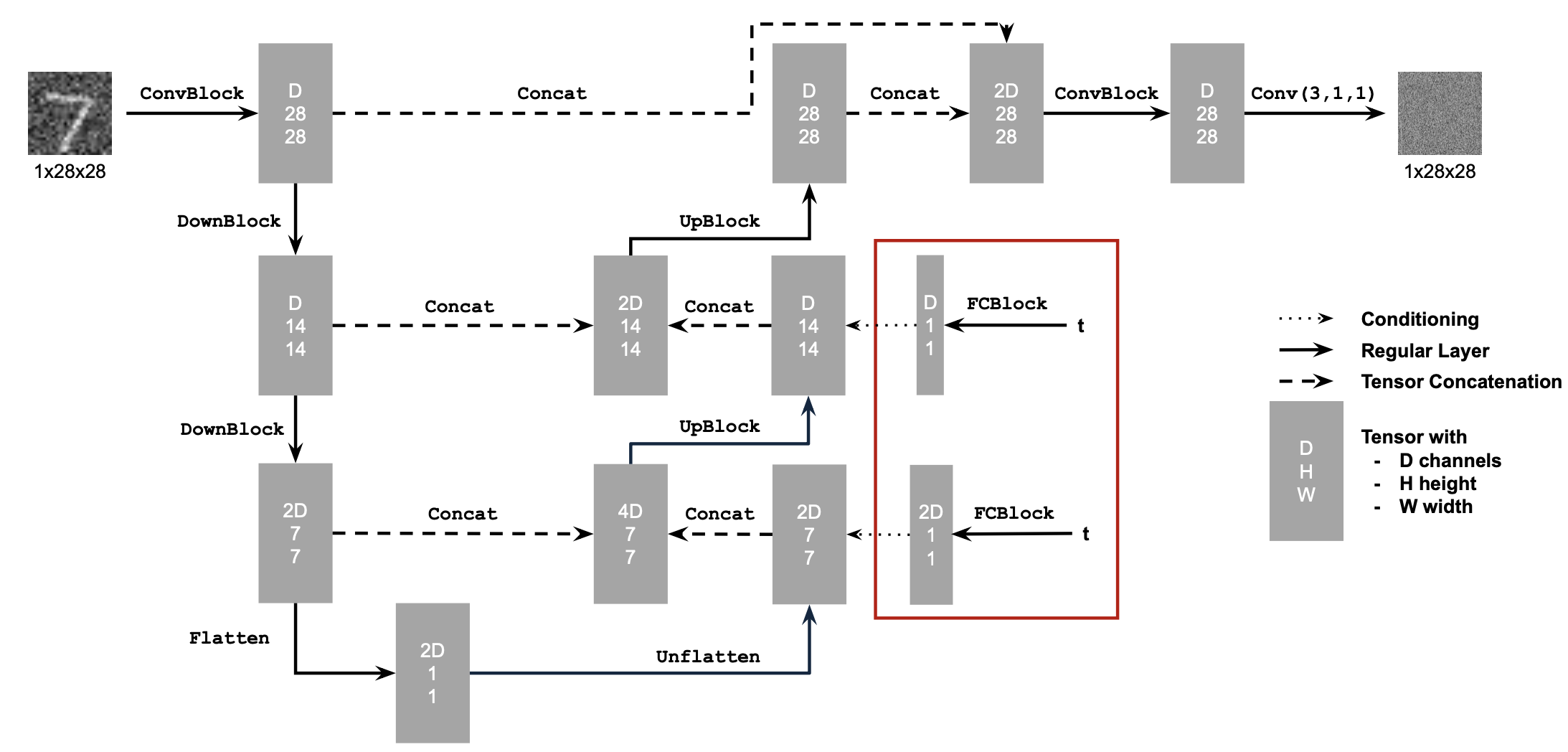
To implement the UNet, I followed exactly the architecture specified in the spec. That is:

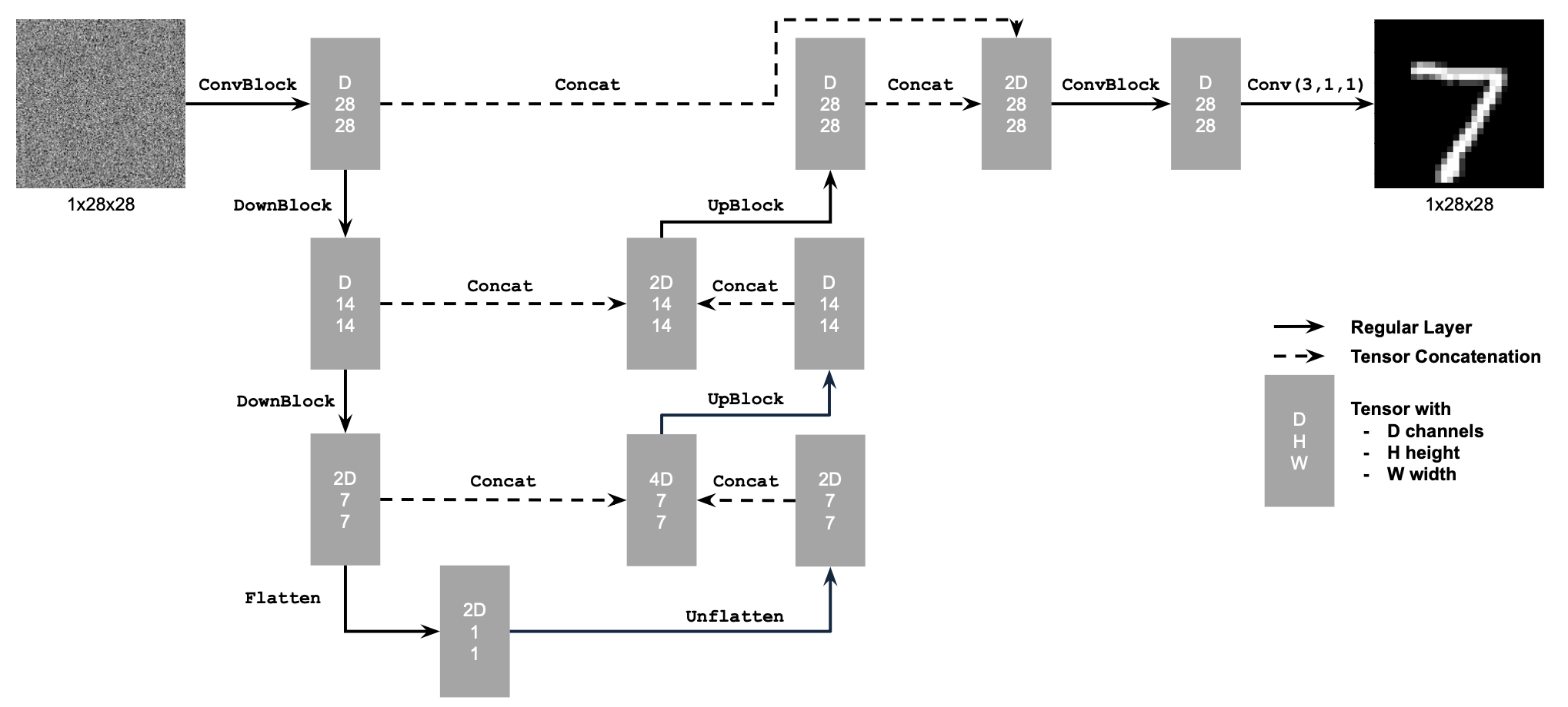
The only twist I made is that in the __init__ function, I compiled the model with nn.Module.compile() to get better performance.

Using the UNet to Train a Denoiser

To train a UNet denoiser, we first need to produce some noised image. When loading the images from MNIST dataset, we pass in a transformation of ToTensor() to convert pixel values into float in [0, 1]. After this, noising is simply adding a same shaped gaussian noise of \(\sigma\) variance. The noised images look like:

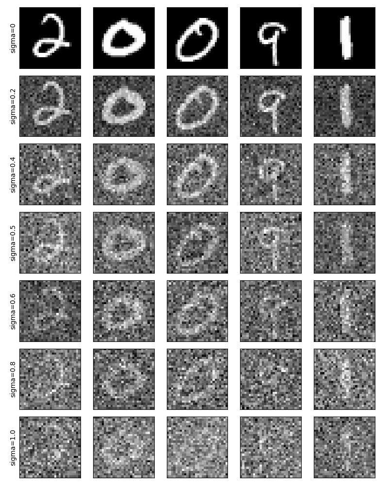
We can then proceed to train a UNet denoiser by simply regressing to the original image given the noised image as input. One thing we should do before start training is normalization. We can normalize the image by subtracting the mean and dividing by the standard deviation. As the image has a range [0, 1], to avoid calculating the true mean and variance, I estimated it to be a uniform distribution in its range and thus have mean of 0.5 and variance of 1/12. After noising the mean is not changed by the variance becomes 1/12+sigma^2.

With the normalization in place, we can start training the model. We train with batch size of 256 for 5 epochs with constant learning rate of 1e-4. This gives a training curve of:

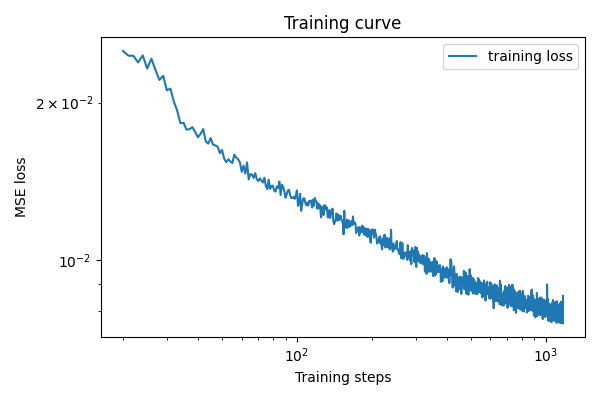
And the denoising results on test set are:

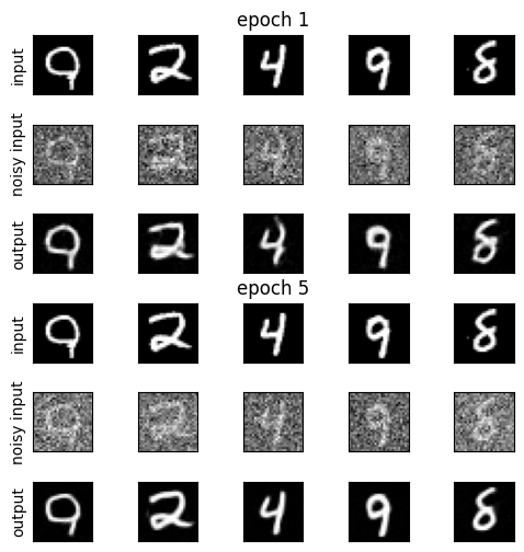
The UNet does a decent job denoising the images.

We can also test on out-of-distribution by adding different values of noise. Note that when we change the sigma, the normalizer’s sigma should not be changed from the training value. The results look like:

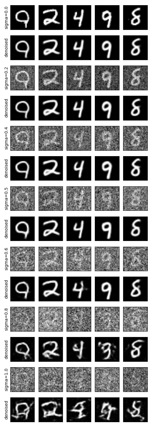
As we can see, the model generalized well to smaller variances but not larger ones.

Training a Diffusion Model

To train a diffusion model, several changes need to be made. Firstly, we need to implement the vairance schedule. The variance schedule defines forward and backward process, namely,

and the sampling (backward) process is defined by:

in our project, \(\beta_t\) is defined to be even interval sequence from 1e-4 to 2e-2. \(\alpha_t\) defined to be \(1 - beta_t\), and \(\hat\alpha_t\) defined to be the cumulative product of \(\alpha_t\).

The last tweak to the denoiser UNet in previous section is that now we need to condition our network by time embedding, which will be elaborate later.

Adding Time Conditioning to UNet

To add time embedding, we add two fully connected blocks (i.e. MLPs) to our model. The embedding they produced are added to the channel dimension of the up-sampled arrays of the unet. The idea is that it will condition the high-level semantics by the time information.

Training the UNet

We train the network with the DDPM algorithm:

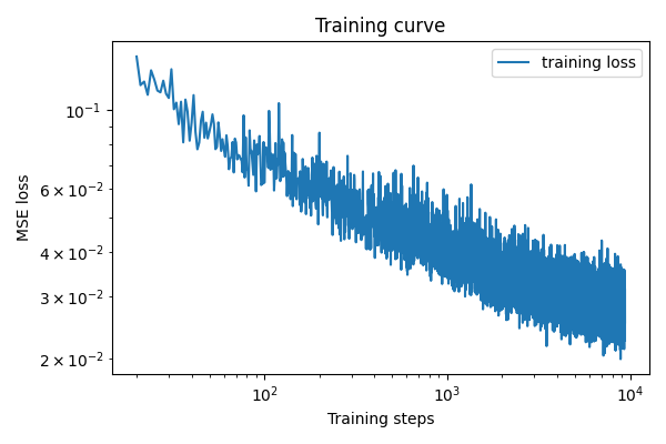
With the normalization in place, we can start training the model. We train with batch size of 128 for 20 epochs with exponentially decayed learning rate starting from 1e-3 and decaying to 1e-4. This gives a training curve of:

Sampling from the UNet

Now we can sample from the UNet with the algorithm layed out in previous section. Using the checkpoints from the 5th and 20th epoch, we obtain the results:

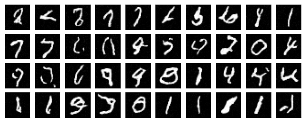
40 images sampled by checkpoint at epoch 5

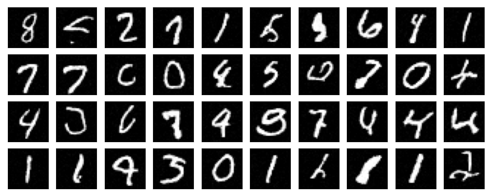
40 images sampled by checkpoint at epoch 20

We see that the results from 20th epoch is better than 5th epoch, but still not perfect.

Adding Class-Conditioning to UNet

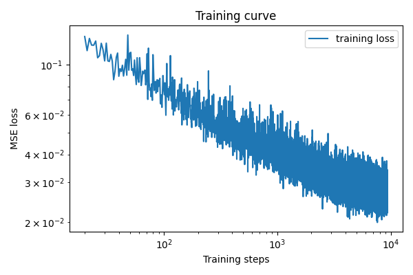
We can improve our modeling by conditioning on the class (digit label). This can be done by adding yet another fully connected block. However, as the input is categorical, it can be fully described by an nn.Embedding module. We initialie a 11 class embedding, where the 11th class is the “unconditioned” class. Then, instead of adding to the up-sampled channels, we multiply them to the up-sampled channels (“gating” in machine learning terms). This is just a design choice and is emprically better (did an ablation and the training loss is lower than adding). The training procedure is identical to the time conditioned one, except for that we feed in classes as the conditions. Furthermore, we generate a Bernoulli random variate with probablity of 0.1 to change the class label to “unconditioned” label for all samples. This allows us to do CFG later. The optimizer parameters are the same as before and it gives a training curve like:

Sampling from the Class-Conditioned UNet

Finally, we can sample from the class-conditioned UNet. The procedure is similar to the previous part, with the twist that we use CFG to improve the conditioning. Using the checkpoints from 5th and 20th epoch, we are able to sample:

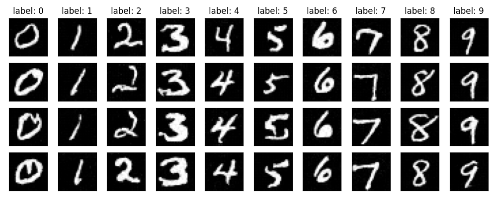
40 images sampled by checkpoint at epoch 5

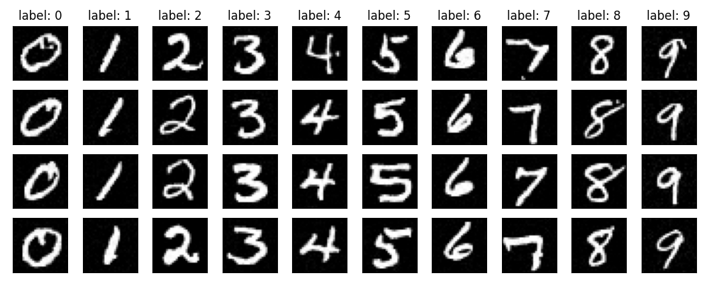
40 images sampled by checkpoint at epoch 20

We see that class conditioning is very strong and successfully forced the sampled images to be the desired class.