Project 4A: Image Warping and Mosaicing!
Warp images to create Mosaics
Introduction
In this project, I implemented image warping (perspective) and created mosaics with it.
Shoot the Pictures
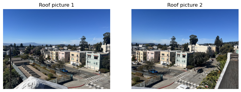
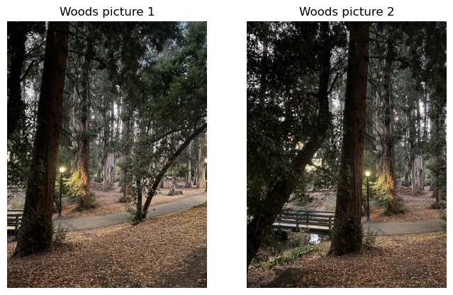
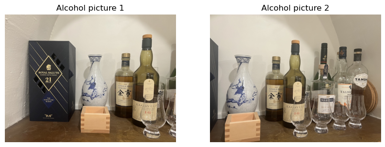
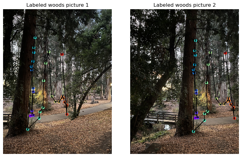
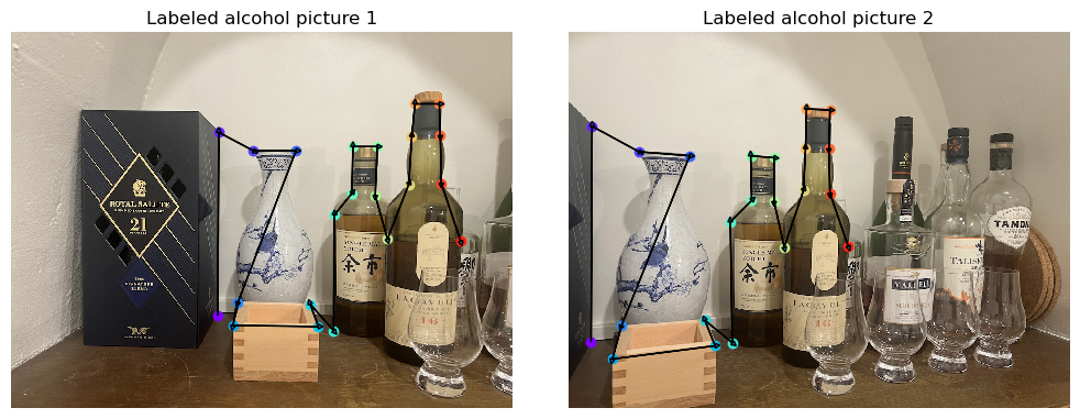
There are two sets of pictures that we need to take. First, we need to take image pairs (or sets) that overlaps significantly to blend them into mosaics. Here, I chose three scenes. The view from my apartment’s roof, the woods next to VLSB, and my alcohol collections. The raw images are presented here:
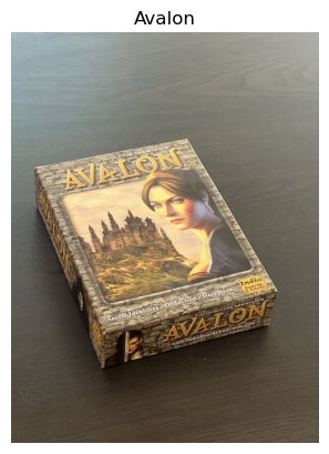
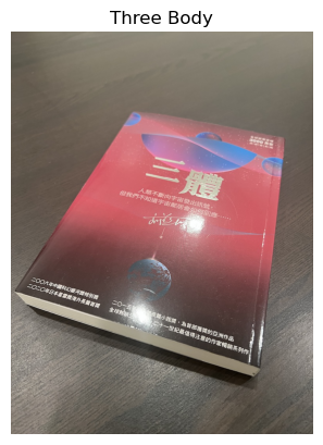
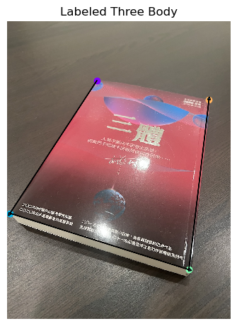
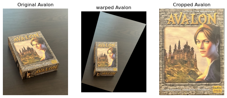
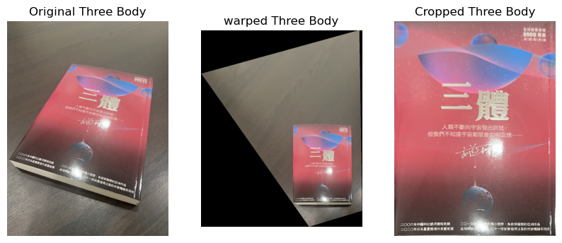
The other set is images with rectangles that we can rectify. Here, I took pictures of a board game’s box and a book. They are presented here:
Recover Homographies
To recover homography, we need to solve:
\[\left[ \begin{matrix} a & b & c \\ d & e & f \\ g & h & 1\\ \end{matrix} \right] \left[ \begin{matrix} x\\ y\\ 1 \end{matrix} \right] = \left[ \begin{matrix} wx'\\ wy'\\ w \end{matrix} \right]\]However, there are nine unknowns here: \(a, b, \dots h, w\). We can remove \(w\) dependency by substituting it with \(w = gx+xy+1\). After algebraic manipulation, it gives the following expression:
\[\left[ \begin{matrix} x & y & 1 & 0 & 0 & 0 & -xx' & -yx' \\ 0 & 0 & 0 & x & y & 1 & -xy' & yy' \end{matrix} \right] \left[ \begin{matrix} a\\ b\\ c\\ d\\ e\\ f\\ g\\ h \end{matrix} \right] = \left[ \begin{matrix} x'\\ y' \end{matrix} \right]\]The calculation used [1] as reference.
The next step is to define the correspondence. This step is very similar to project 3, and I reused the infrasturcture. One difference is that to get more stable homographies, we can use overcomplete system. We have eight unknowns, and each pair of points gives two constraints. This means that four point should be enough. However, as labeling is done by human and there is always error in labeling, this problem is analogus to Ridge regression. In Ridge regression, the more data points we have, the more accurate the regressed value becomes. Therefore, we label many corespondance points, and use np.linalg.lstsq to solve for the best fit. However, for image rectification, as the only four points we know are the four corners of the rectangle, we can’t do better than four points.
The labeled images are presented below:
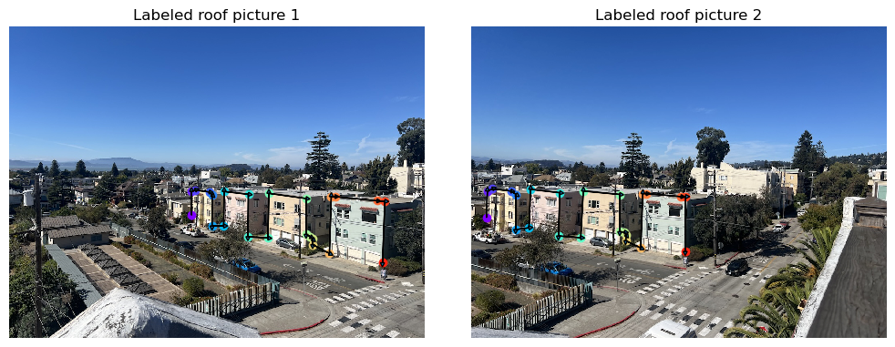

For a sanity check, we can try mapping the correspondence points with the Homography we got and compute the sum of squared distances between the points, and divide them by number of points minus either (dofs). This is known as the reduced Chi-squared statistics (with a 2D standard normal noise model). The reduced chi-squared of the roof images is 6.5, which suggests an average 2~3 pixel difference, which is pretty good.
Warp the Images
Now we can proceed to wraping the images. As in project 3, the best way is to use the inverse mapping and interpolate in the original image. This requires knowing the exact inverse of the transformation. Fortunately, the homography \(H\) in most cases in invertable, and we can simply invert it to get the pixel locations in the original image. Therefore, the algorithm goes as follows: first, we use \(H\) and wrap the four corners of the original images to the wrapped coordinates. In the wraped coordinantes, we create a polygon mask using skimage.draw.polygon. We know that the wraped image is going to fill the polygon as projections preserve straight lines. Note that this polygon can have negative coordinantes and therefore we need to shift the image when necessary. Then, we compute \(H^{-1}\) and use that to get the pixel locations in the original coordinantes. Bilinearly interpolate the pixel values, and then fill them into the wraped coordinantes.
Image Rectification
Now with the warping function implemented, we can proceed to image rectification. Note that the board game box and the book have a known aspect ratio of 3 by 4, we can manually create the correspondence. This gives:
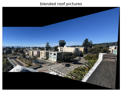
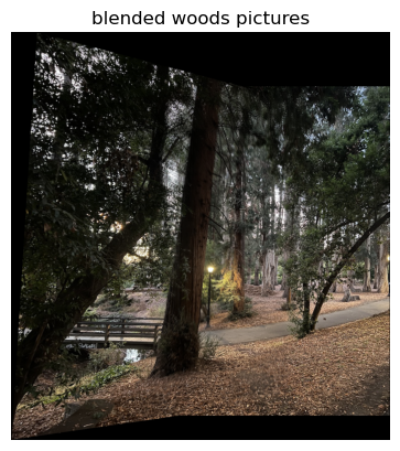
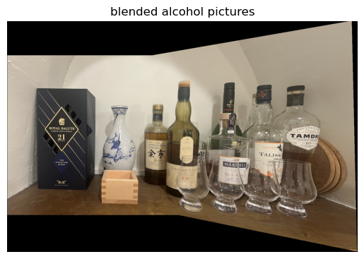
Blend the images into a mosaic
The last part is to blend images into mosaic. There are two technical difficulties. First, as mentioned before, sometimes the warped coordinantes are negative. Though in image rectification we can simply shift it by constant amount to make all of them positive, it ruins the alignment in the case of blending. Therefore, we need to pad the images such that they are realigned. The other issue is that if we naively overlay the two images, there will be sharp boundary effects that can be observed with eyes. The way around is to assign an \(\alpha\) to each pixel by one minus its relative distance to the center of the image (here I used infinite norm so that boundaries have the same value of \(\alpha\)). Then, we blend by taking the weighted average of the two images given by weights \(\alpha\). This gives a smooth transition, and the results are shown below: The labeled images are presented below: