Project 4: Image Warping and Mosaicing!
Stitching Photo Mosaics
Introduction
In this project, I implemented image warping (perspective), auto feature detection and matching, and created mosaics with it.
Shoot the Pictures
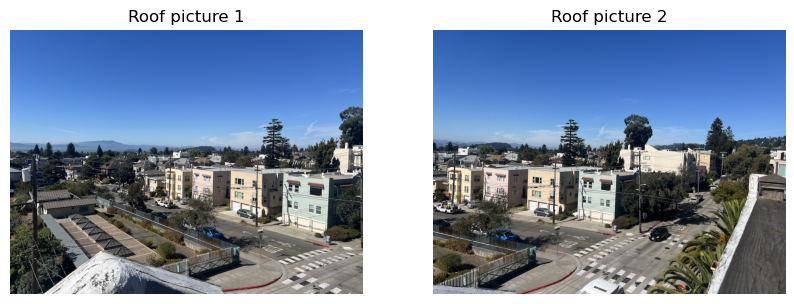
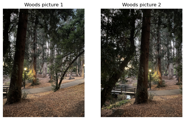
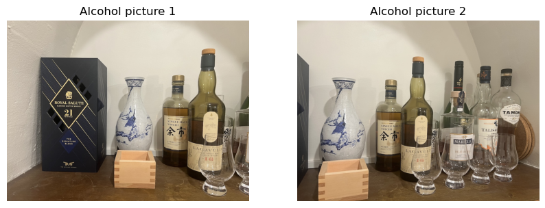
There are two sets of pictures that we need to take. First, we need to take image pairs (or sets) that overlaps significantly to blend them into mosaics. Here, I chose three scenes. The view from my apartment’s roof, the woods next to VLSB, and my alcohol collections. The raw images are presented here:
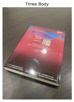
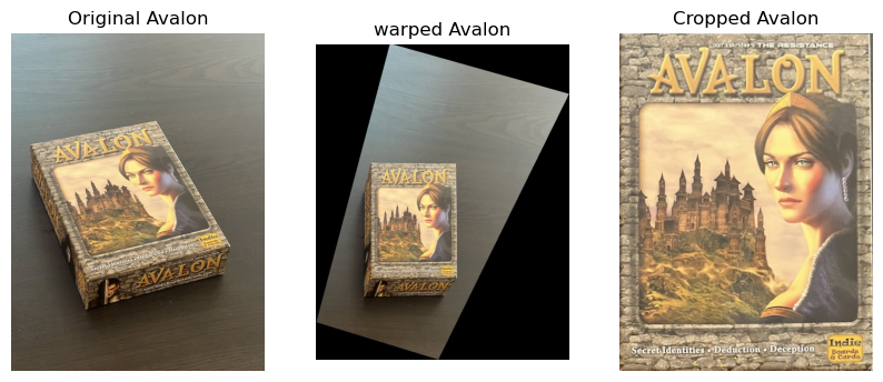
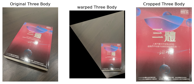
The other set is images with rectangles that we can rectify. Here, I took pictures of a board game’s box and a book. They are presented here:

Recover Homographies
To recover homography, we need to solve:
\[\left[ \begin{matrix} a & b & c \\ d & e & f \\ g & h & 1\\ \end{matrix} \right] \left[ \begin{matrix} x\\ y\\ 1 \end{matrix} \right] = \left[ \begin{matrix} wx'\\ wy'\\ w \end{matrix} \right]\]However, there are nine unknowns here: \(a, b, \dots h, w\). We can remove \(w\) dependency by substituting it with \(w = gx+xy+1\). After algebraic manipulation, it gives the following expression:
\[\left[ \begin{matrix} x & y & 1 & 0 & 0 & 0 & -xx' & -yx' \\ 0 & 0 & 0 & x & y & 1 & -xy' & yy' \end{matrix} \right] \left[ \begin{matrix} a\\ b\\ c\\ d\\ e\\ f\\ g\\ h \end{matrix} \right] = \left[ \begin{matrix} x'\\ y' \end{matrix} \right]\]The calculation used [1] as reference.
The next step is to define the correspondence. This step is very similar to project 3, and I reused the infrasturcture. One difference is that to get more stable homographies, we can use overcomplete system. We have eight unknowns, and each pair of points gives two constraints. This means that four point should be enough. However, as labeling is done by human and there is always error in labeling, this problem is analogus to Ridge regression. In Ridge regression, the more data points we have, the more accurate the regressed value becomes. Therefore, we label many corespondance points, and use np.linalg.lstsq to solve for the best fit. However, for image rectification, as the only four points we know are the four corners of the rectangle, we can’t do better than four points.
The labeled images are presented below:
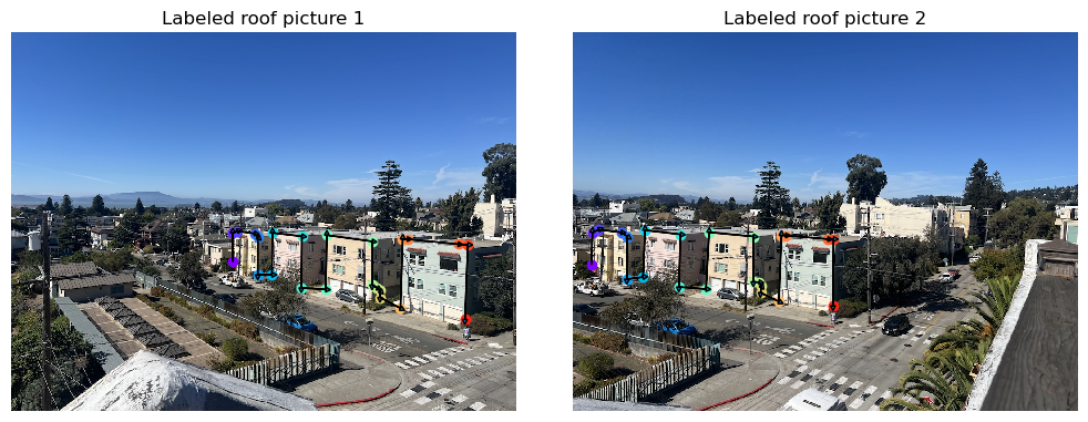
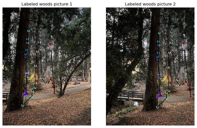
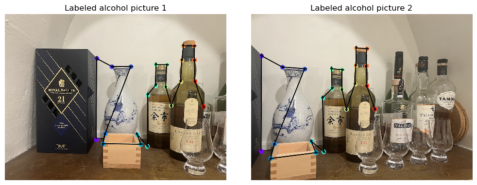
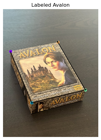
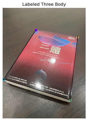
For a sanity check, we can try mapping the correspondence points with the Homography we got and compute the sum of squared distances between the points, and divide them by number of points minus either (dofs). This is known as the reduced Chi-squared statistics (with a 2D standard normal noise model). The reduced chi-squared of the roof images is 6.5, which suggests an average 2~3 pixel difference, which is pretty good.
Warp the Images
Now we can proceed to wraping the images. As in project 3, the best way is to use the inverse mapping and interpolate in the original image. This requires knowing the exact inverse of the transformation. Fortunately, the homography \(H\) in most cases in invertable, and we can simply invert it to get the pixel locations in the original image. Therefore, the algorithm goes as follows: first, we use \(H\) and wrap the four corners of the original images to the wrapped coordinates. In the wraped coordinantes, we create a polygon mask using skimage.draw.polygon. We know that the wraped image is going to fill the polygon as projections preserve straight lines. Note that this polygon can have negative coordinantes and therefore we need to shift the image when necessary. Then, we compute \(H^{-1}\) and use that to get the pixel locations in the original coordinantes. Bilinearly interpolate the pixel values, and then fill them into the wraped coordinantes.
Image Rectification
Now with the warping function implemented, we can proceed to image rectification. Note that the board game box and the book have a known aspect ratio of 3 by 4, we can manually create the correspondence. This gives:
Blend the Images into a Mosaic
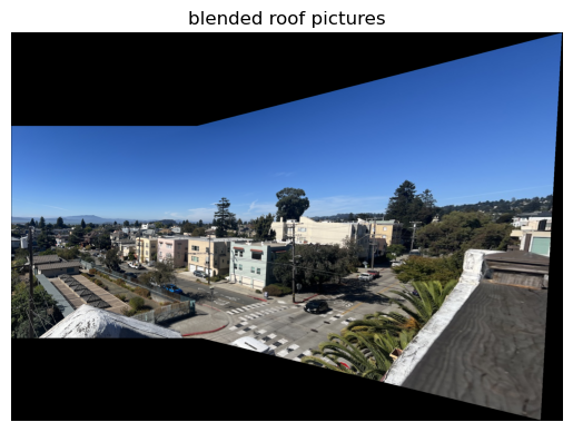
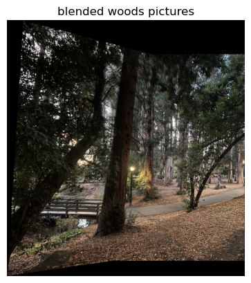
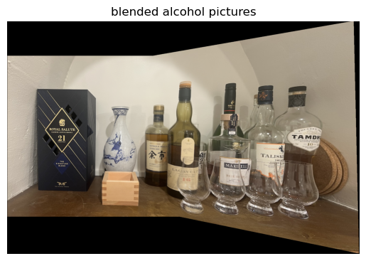
The last part is to blend images into mosaic. There are two technical difficulties. First, as mentioned before, sometimes the warped coordinantes are negative. Though in image rectification we can simply shift it by constant amount to make all of them positive, it ruins the alignment in the case of blending. Therefore, we need to pad the images such that they are realigned. The other issue is that if we naively overlay the two images, there will be sharp boundary effects that can be observed with eyes. The way around is to assign an \(\alpha\) to each pixel by one minus its relative distance to the center of the image (here I used infinite norm so that boundaries have the same value of \(\alpha\)). Then, we blend by taking the weighted average of the two images given by weights \(\alpha\). This gives a smooth transition, and the results are shown below: The labeled images are presented below:
Detect Corners
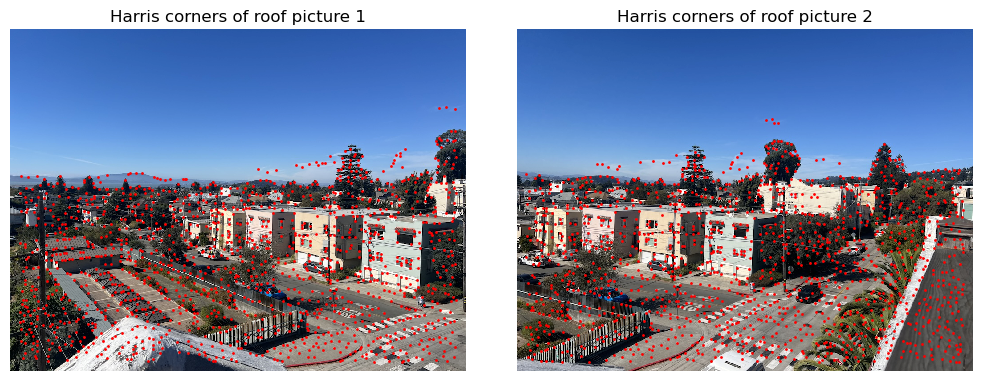
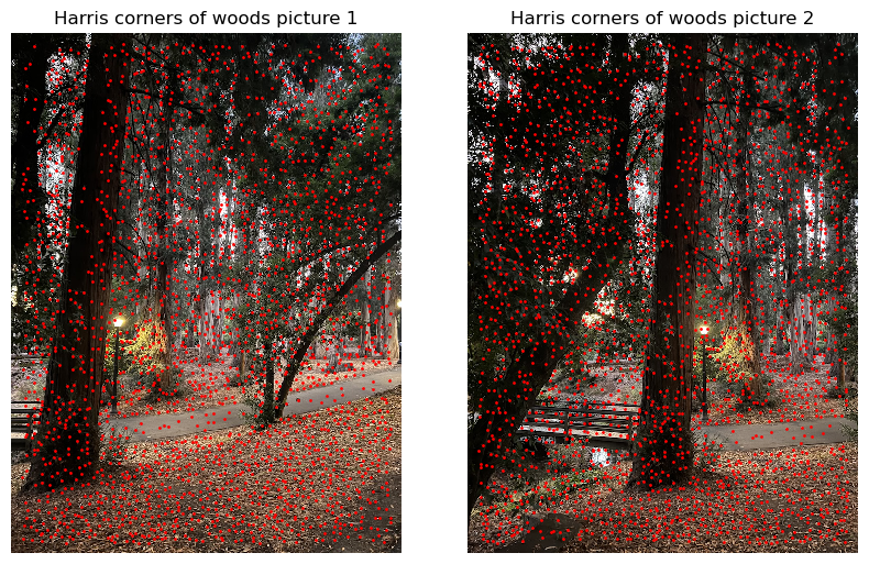
The first step toward auto-alignment is to detect the corners. This is done by running the Haris corner detection algorithm with skimage.feature.corner_harris. Furthermore, following the sample code provided in the project spec, I did three post processing. First, I ran skimage.feature.peak_local_max to get the locations that is a local maximum (with minimum distance one). Removing non-locally-maximal points is important as the NMAS algorithm that will be run later scales quadratically with the number of corners. I subsequently applied a threshold to make sure that there are no “corners” on supposedly flat region such as sky. Matching with corners induced by noise will just lower the quality. The cut is 1e-3 which is very low to preserve the most features for the next step. Finally, I applied a selection to remove any corners within 20 pixels from the edges. This is because when we build the feature descriptors we need to sample a 40 by 40 window, which is impossible if they are within 20 pixels. The Harris corners are visualized as following:
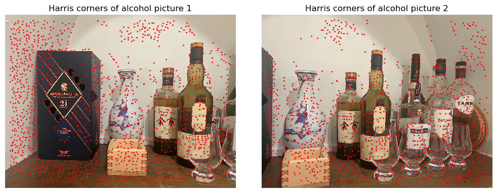
The next step is to implement Adaptive Non-Maximal Suppression (ANMS). The definition of suppresion radius for a point is:
\[r_i = \min_{j} ||x_i-x_j||_2,\mbox{ s.t. } f(x_i) < c_{robust} f(x_j)\]In other words, it is the radius of the nearest pixel where the “corner strenth” \(f\) is \(1/c_{robust}\) stronger than the pixel of interest. Following the paper “Multi-Image Matching using Multi-Scale Oriented Patches” [2], \(c_{robust}=0.9\). This algorithm is implemented by simply taking the N corners detected by Harris algorithm and compute the distances of all pairs of them, constructing a N by N matrix. Then, for the entries that are not able to suppress the i-th corner (\(f(x_i) \geq c_{robust} f(x_j)\)), we set the corresponding distance entry to be inf. Then we take per-row minimum to get the suppresion radius for each corner. Finally, sort the corners by their suprresion radius and return the desired number of corners. The result is presented below:
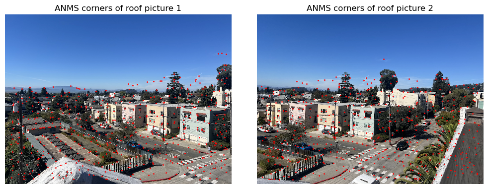
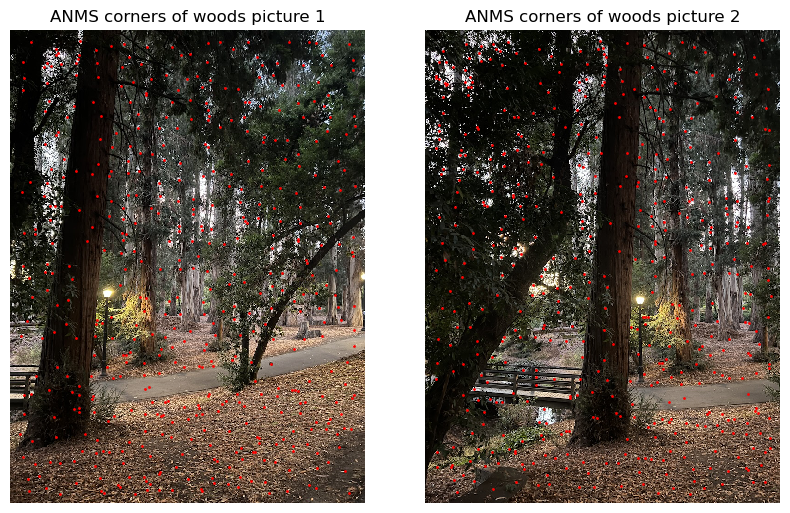
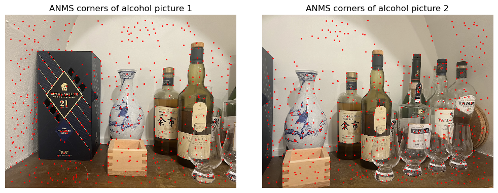
Here, number of corners returned is 500. Other numbers can be used, I just followed the number used in the paper. The radis of each picture is:
| roof | woods | alcohol | |
|---|---|---|---|
| picture 1 | 19.03 | 24.70 | 22.02 |
| picture 2 | 19.10 | 25.00 | 20.25 |
Feature Descriptor Extraction
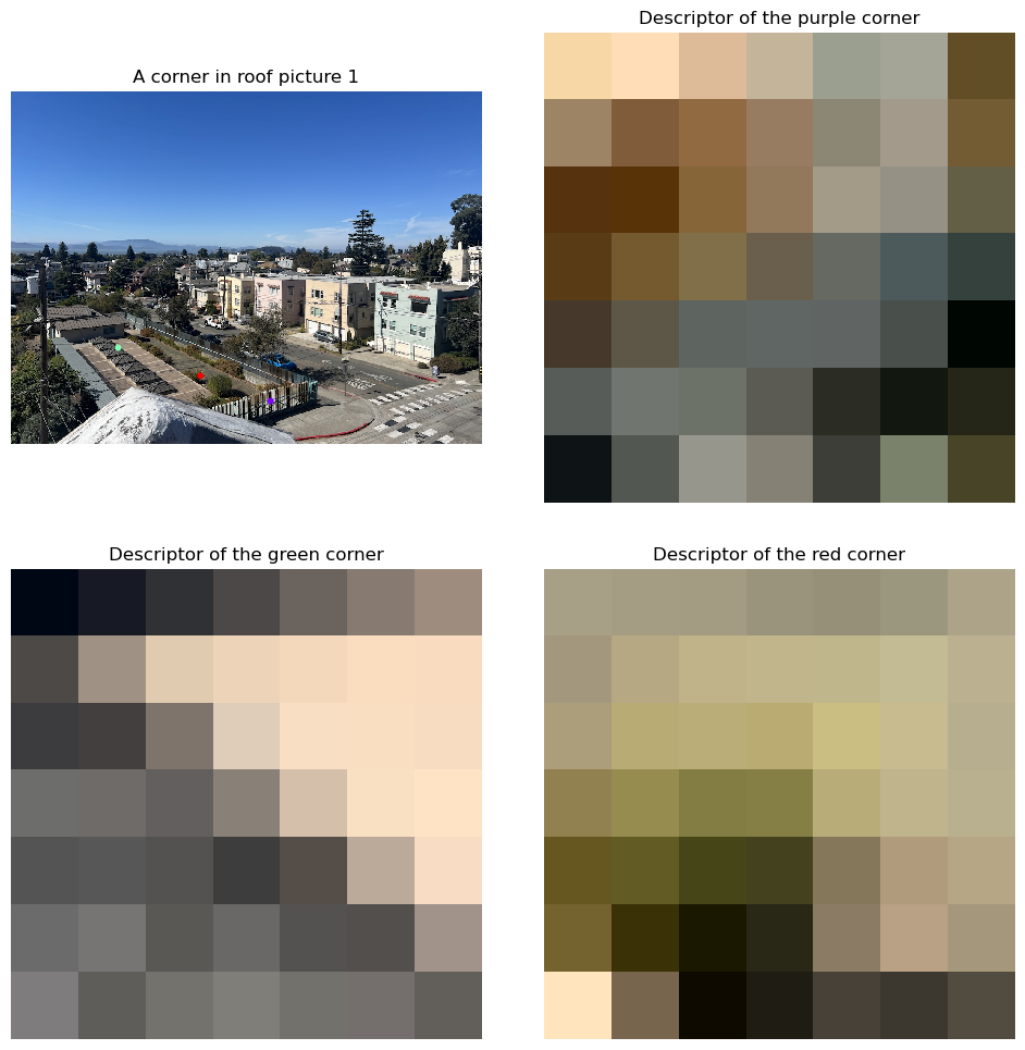
Now the task is to extract the feature descriptors. This involves two steps. First, we need to downsample the image to get the low frequency information. I choose to use Gaussian filter to ahieve this. Note that since we are downsampling by a factor of 5, I choose the standard deviation of the kernel to be five pixels. After low-pass filter, we can safely downsample the image without worrying about aliasing. This is done by sampling a eight by eight grid centered around each corner with a stride 5. The next step involves normalizing each descriptor. Since my pictures are colored, I think the color information is important for getting better homographies. The descriptors are therefore normalized to have zero mean and unit variance along both spatial and color channels. Here I visualized a few examples, they are renormalized to have minimum of 0 and maximum of 1 for visualization purposes:
Feature Matching
Now we proceed to matching these feature descriptors. Given two sets of feature descriptors, I compute the L2 distances squared between each pair of them. Then, for each descriptor in the first set, sort the other set of descriptors by their distances. Define score as the smallest distance divided by the second smallest distance. This score is bounded between zero and one, and only pairs with score less than 0.4 is accepted. The threshold is selected based on this plot from [2]:
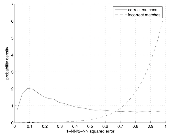
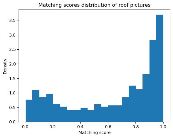
The two distribution also looks similar to each other, which confirms the validity of this method.
RANSAC
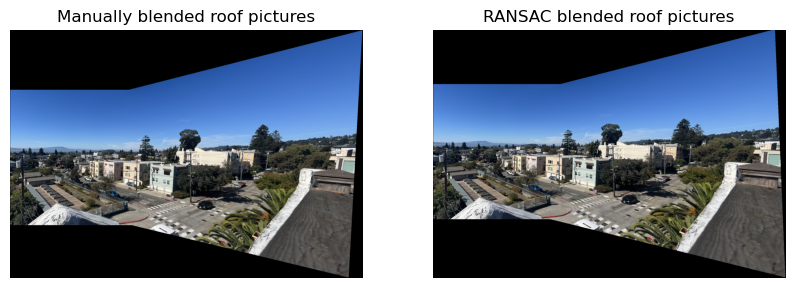
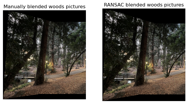
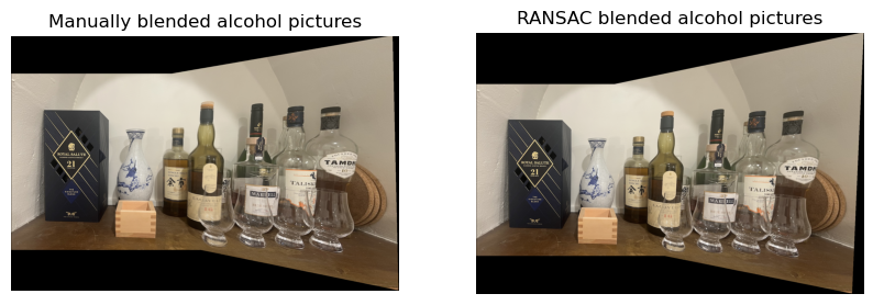
Finally, as there will still be false matches after the feature space based rejection method, we need to come up with an algorithm that can use only the inliers. This is the random sample consensus algorithm. The algorithm starts by randomly choosing four points and compute a homography with it. With sufficiently high rate of true matches, this random sample should have fairly high chance to be four true matches. We then use the homography to map the coordinates of each feature to another image’s coordinate system. For each pair of matched features, the loss function is the L2 distance squared. For any sample with loss above the threshold, they are consider “outliers” and will be excluded. We record the number of inliers, and if there are more than specific fraction of the matched features are inlier, we consider this homography as “good” and record the MSE of inliers of this homography. This process is repeated N=1000 times to get the best homographies and set of inliers. Traditionally, the best fit (homography) is returned and used. Here, instead, I return the best homography’s inlier set and use all of them to compute a better homography with least square. The error threshold is chose to be 2 pixels to match with manual labeling precision (the chi square value before), and the inlier fraction is chosen to be 0.5. With the homography, we can automatically blend the pictures and the results are presented below. The manually blended version is also provided for comparison.
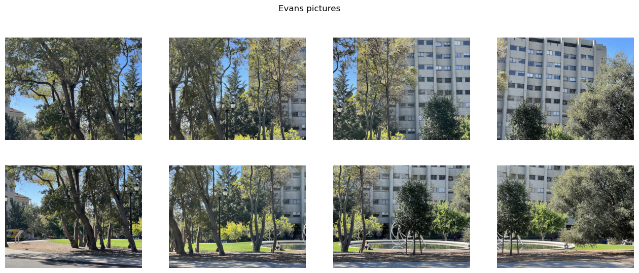
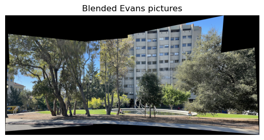
Blend Multiple
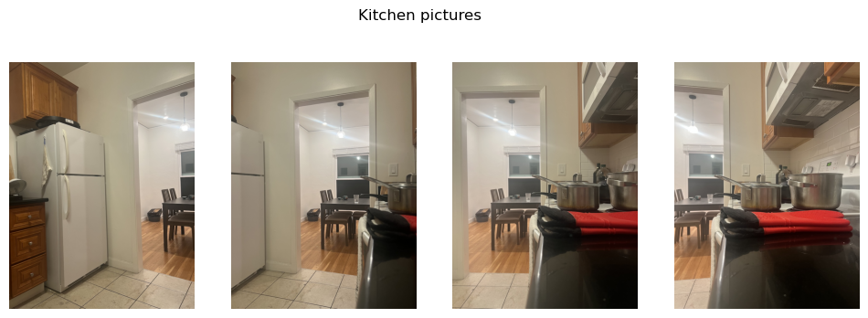
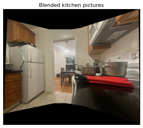
Finally, we can try blending multiple pictures. This can done by iteratively blending two pictures together. This requires two modification to our previous implementation. First, instead of having a fixed matching fraction of 0.5 for RANSAC, we need to gradually lower it as the blended image becomes larger there will be less overlap between them. I choose the fraction to be \(1/\mbox{#images blended}\). The next thing to modify is alpha blending. We need to preserve the alpha channel throughout the blending process as the blended images contains paddings, and if we naively feed that into the blending function they will also recieve finite alpha value which will yeild incorrect results on boundaries. Finally, the order of blending also matters. As a hard requirement, the new picture to be blended in must have overlap with the already blended portion. It is in general the best practice to slowly “grow” the image from the center of the panarama.
References
[1] Project 4 - Alec Li Stitching Photo Mosaics
[2] M. Brown, R. Szeliski and S. Winder, “Multi-image matching using multi-scale oriented patches,” 2005 IEEE Computer Society Conference on Computer Vision and Pattern Recognition (CVPR’05), San Diego, CA, USA, 2005, pp. 510-517 vol. 1, doi: 10.1109/CVPR.2005.235.