Project 3: Face Morphing! | Ryan Liu's Homepage

Introduction

In this project, I implemented face morphing through triangulation, affine wrapping, and cross-dissolve.

Part 1. Defining Correspondences

Before wrapping the images, we first need to define the “correspondences” of the images. This is because the geometries of different people’s faces differ a lot and naively cross-dissolving the images will result in bad outputs. Therefore, we need to define the points that should be morphed into each others. I wrote a utility function based on plt.ginput to get user defined anchor points. Since the order matters, I also devised a visulization tool to show the user the order of points that were used to label the other images.

The four corners are not added by the user during labeling. They are added when the points are loaded from the disk. After using the Delaunay triangulation, these points give a triangulation of:

Part 2. Computing the “Mid-way Face”

With the correspondences, we can start morphing the images. The first task is to calculate the inverse affine mapping from the target triangulation to the original triangulation. There are two methods to do this. First, we can solve for the affine mapping between two triangles:

\[\left[ \begin{matrix} a & b & c\\ d & e & f \end{matrix} \right] \left[ \begin{matrix} p_x\\ p_y\\ 1 \end{matrix} \right] = \left[ \begin{matrix} q_x & q_y \end{matrix} \right]\]

Here \(p\) and \(q\) are the corresponding points of two triangles. There are three points in total, therefore giving three such constraints each with two equations. Which gives:

\[\left[ \begin{matrix} p_{x1} & p_{y1} & 1 & 0 &0 &0\\ 0 &0 &0 & p_{x1} & p_{y1} & 1\\ p_{x2} & p_{y2} & 1 & 0 &0 &0\\ 0 &0 &0 & p_{x2} & p_{y2} & 1\\ p_{x3} & p_{y3} & 1 & 0 &0 &0\\ 0 &0 &0 & p_{x3} & p_{y3} & 1\\ \end{matrix} \right] \left[ \begin{matrix} a\\ b\\ c\\ d\\ e\\ f \end{matrix} \right] = \left[ \begin{matrix} q_{x1}\\ q_{y1}\\ q_{x2}\\ q_{y2}\\ q_{x3}\\ q_{y5}\\ \end{matrix} \right]\]

Which can be solved with np.solve

Another approach is to transform everything to the barycentric coordinantes. The barycentric coordinantes are defined as the signed area of the three triangles formed by connecting the point to the three points forming the triangle. Concretely, the transformation of \((x, y)\) to its barycentric coordinantes can be computed as:

\[\left[ \begin{matrix} x_1 - x_3 & x_2 - x_3 \\ y_1 - y_3 & y_2 - y_3 \end{matrix} \right] \left[ \begin{matrix} \lambda_1 \\ \lambda_2 \end{matrix} \right] = \left[ \begin{matrix} x - x_3\\ y - y_3 \end{matrix} \right]\]

Similarly, this can be solved by np.solve. The inverse transformation is easy to compute; just do matrix multiplcation then add \((x_3, y_3)\) back can do that. Note that since this transformation can be written as a linear system (with addition/subtraction), it is affine by definition.

With the wrapping function implemented, the process of computing the midway face is easy. First, we compute the mid-way geometry by taking the arithmetic average of the two sets of correspondence points. Then, triangularize it with the scipy.spatial.Delaunay algorithm. For each triangle, we use skimage.draw.polygon to get the pixels coordinantes in the mid-way geometry covered by each triangle. Depending on the transformation method one wants to use, solve for either the affine transformation from the mid-way geometry coordinantes to the original picture geometry or the barycentric coordinantes of the pixels in the triangle. With the affine transformation/barycentric coordinantes, we then map them back into the original picture’s coordinante system by applying the affine transformation or convert the barycentric coordinantes back into Cartesian coordinantes. With the coordinantes in the original picutres coordinante system, since they can be non-integer, we perform bilinear interpolation to get the pixel value corresponding to the point. Finally, we average the pixel values queried from both images and fill that into the corresponding pixel location in the mid-way picture. The mid-way picture of Soohyun and I, along with the wrapped picture of both, is presented below:

Part 3. The Morph Sequence

Now we want to compute the morphing sequence. The implementation is very simple; we just need some slight modification from the previous part. First, we compute the triangulation based on the target picture. This is because we want the best-looking final output not the mid-way one (if images are in good alignment the triangulation should not be differnet). Secondly, instead of calculating the mid-way geometry defined by the arithmetic average, we interpolate between the two images with warp_frac. The wrapping process is identical. With the wrapped images, we again interpolate between the two images’ pixel values with dissolve_frac to obtain the cross-dissolved output. One edge case is that if warp_frac and dissolve_frac are both zero or one, giving the original images can offer some speed up as we knew the output (original images). The final product looks like:

In case of the gif file doesn’t load on the website. follow this link to view the GIF.

Part 4. The “Mean face” of a population

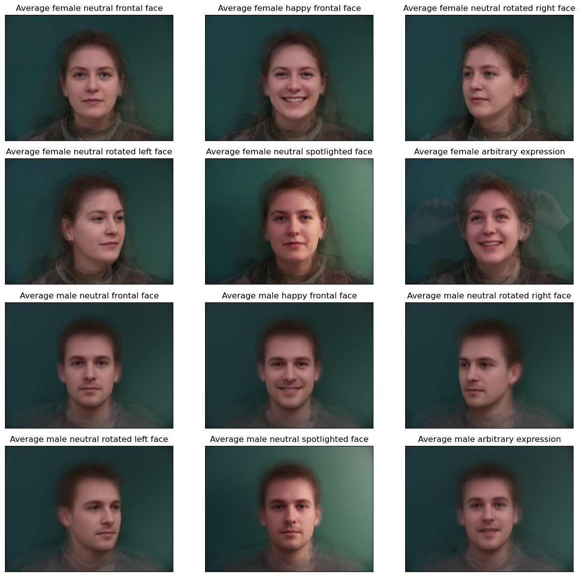
Next, we proceed to calculating the “mean face” of the population. To do this, I used the IMM Face Database, which has 240 annotated monocular images of 40 different human faces. I wrote a simple tool to parse the .asf file which contains the annotation information. Then, for each group of the faces (they grouped the faces according to the gender and image types), we calculate the average points and triangulate accordingly. Then, we wrap all faces of that group into the average geometry and take the pixel value average. The result looks like:

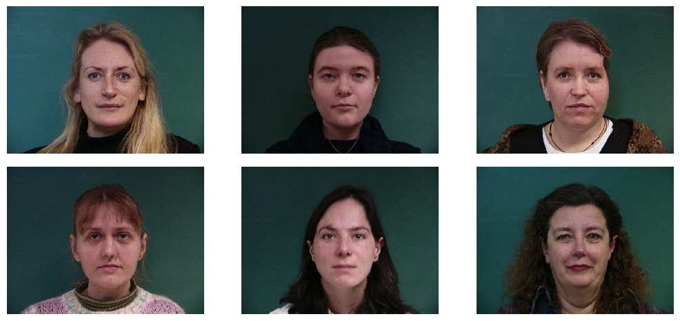
We can try wrapping individual faces from the database into the average faces. Here are the female neutral faces wrapped into their agerage geometry:

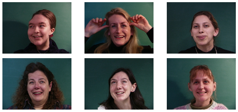
and the arbitraty faces into average:

We can try wrapping my own face

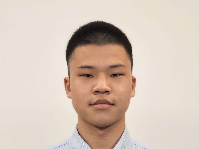
into their average geometry:

Or their average faces into my geometry:

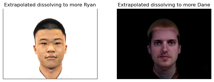
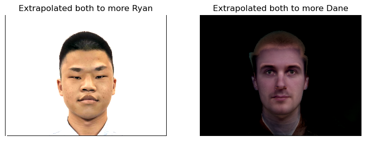
Part 5. Caricatures: Extrapolating from the mean

Finally, to create some funny picture, instead of interpolating, we can extrapolate. That is, to make me more “Ryan” compared with the average or to make the average faces less “Ryan.” This can be easily achieved by changing warp_frac and dissolve_frac to not be in [0, 1].

For example, we can try wrapping both images (Ryan amd Danes’ average) to the average geometry of us, and extrapolate the pixel value (here I setdissolve_frac to -0.5 and 1.5):

Or we can try wrapping one of the images (Ryan amd Danes’ average) to the extrapolated geometry of the other, and average the pixel value (here I setwrap_frac to -0.5 and 1.5):

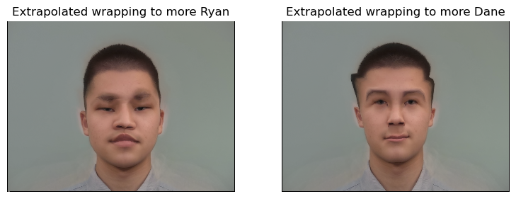
Or maybe both, setting dissolve_frac and wrap_frac to -0.5 and 1.5:

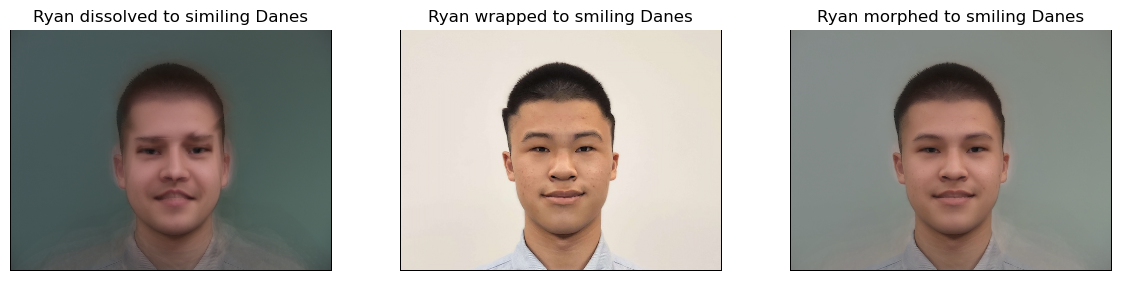
Bells and Whistles. Changing expressions and gender

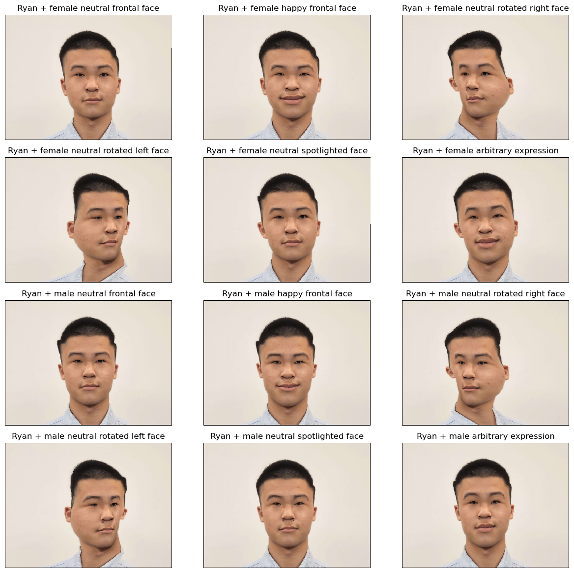
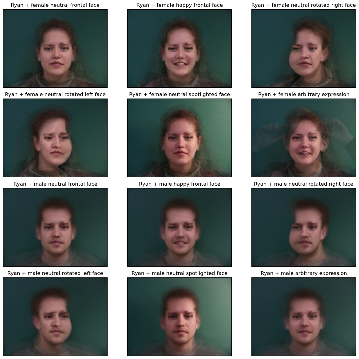
To get more interesting results, we can try morphing to pictures with different expressions and gender. For expressions, I morph my neutral picture into the smiling Danes. I tried fixing my own geometry and cross-dissolving the smiling Danes’ pixel value to my geometry (dissolve_frac is set to 0.8), the other way around (wrap_frac to 0.8), or both (wrap_frac=dissolve_frac=0.5). Here are the results:

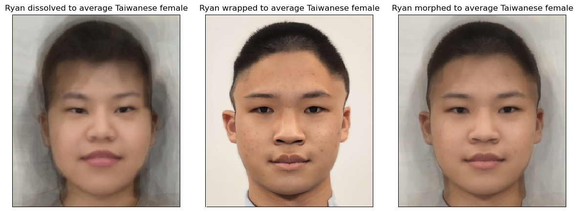
Or we can try changing the gender. Here I used the average Taiwanese female’s faces from this website. The average face looks like:

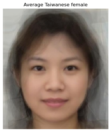
and following the same procedure, I tried three different morphing schemes:

References

M. B. Stegmann, B. K. Ersbøll, and R. Larsen. FAME – a flexible appearance modelling environment. IEEE Trans. on Medical Imaging, 22(10):1319–1331, 2003