Project 2: Fun with Filters and Frequencies!

Inroduction

In this project, I explored the use of frequencies and filters in image processing, and created interesting images with image filtering, morphing, and blending.

Part 1: Fun with Filters

Part 1.1: Finite Difference Operator

First, we have the input image as:

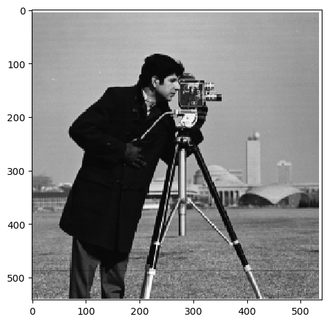
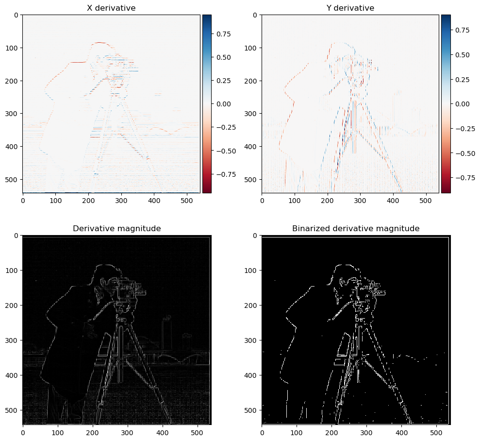
Next, we define the two differentiation operators. Differentiation is approximated by finite differences in descrete case. This is done by taking the differences in respective directions. We have: \(D_x = [[1], [-1]]\) and \(D_y = [[1, -1]]\). We then convolve the operators with the image. Since the image is gray scale, we can simply use convolve2d from scipy. The mode is selected to be same to produce a same-sized image. The boundary condition uses symm to reflect the boundary pixels such that no peculiar gradients appears there. The magniude of the derivative is calculated by \(\sqrt{(\partial_x I)^2+(\partial_y I)^2}\). We also normalize it to have maximum one for visualization. To get clean edges, we also binarize the image with a threshold of the 97 percentile.

Part 1.2: Derivative of Gaussian (DoG) Filter

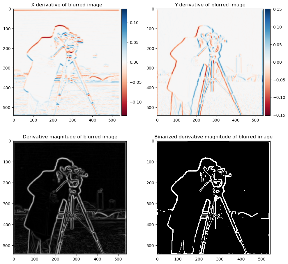
First, we create gaussian kernels by calculating the radius from center of the square. This is achieved by laying out x and y in the unit of sigma on a grid with np.linspace. After that, r is calculated by np.hypot and subsequently fed into the pdf of the normal distribution. Finally, the kernel is normalized to sum to one. We then blur the image with this Gaussian kernel:

Similar to previous part, we differentiate the blurred images. This time the threshold is the 92 percentile of the magnitudes. We see that the edges (high intensity regions) are wider, while the weird artifacts of derivative seen in previous part is no longer presenting.

Alternatively, instead of taking the derivative of the blurred image, we can take the derivative of the gaussian kernel and apply them to the image. Here is the visualization of the derivative of gaussian kernel:

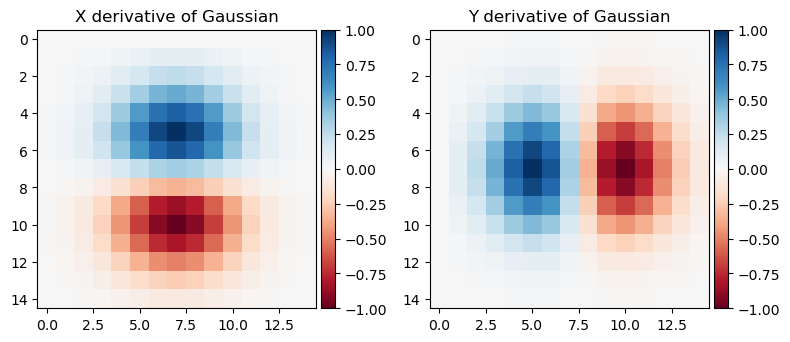
With this Derivative of Gaussian (DoG) filter, we get:

Even though numerically the DoG and the derivative of blurred image are sligtly different due to some boundary effects, the visual effect of the two methods (blurred derivative and derivative of Gaussian) are almost identical.

Part 2: Fun with Frequencies!

Part 2.1: Image “Sharpening”

To mask out low frequency part, we can use a combination of identity transformation (impulse filter) and a low-pass filter (gaussian). Furthermore, since we want the sum of the original image and the high frequency part to obtain a “sharpened” image, we need an additional identity transformation. That is, a negative Gaussian filter and a 2x impulse filter. Convolving with this filter, we get:

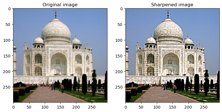
For another image of my choice:

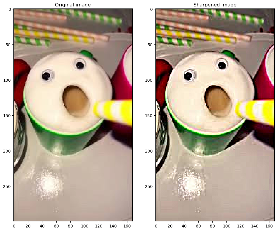
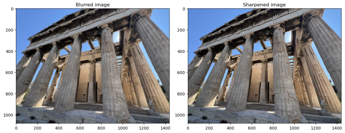
Notice that unsharp_mask_filter can result in non-normalized images, I also clip the values that are too big/small before visualizing them. As we can see, the images became “sharper,” especially around the edges. For evaluation, I chose a high-fidelity picture of the temple of Hephaestus in Athens. Blur it then sharpen it. We can see the texture of the architecture has been sharpened a lot to be more visible.

Part 2.2: Hybrid Images

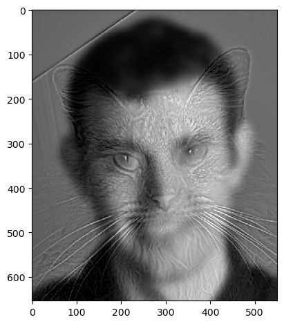
In order to make hybrid (morphed) images, we need todefine two filters. The low pass filter is a gaussian filter of size 51. The high pass filter is a combination of negative gaussian filter and an impulse filter with a size of 21. The numbers are tuned to obtain best visual effects. To reproduce the example in the documentation, we convolve Derek with low pass filter and nutmeg with high pass filter, overlay them, and crop the edges away:

Now, as the implementation is pretty successful, we proceed to my favorite result. This is a pair of funny pictures of Alex, my 162 group mate. The pictures were taken during the celebration of our completion of the final project. The happy one was our original group pic, and the sad one was when we were thinking about all the pain we went through throughout the semester.

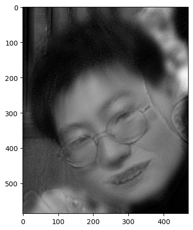
Covered by the smiles, it was the deep frustration we got throughout the class!

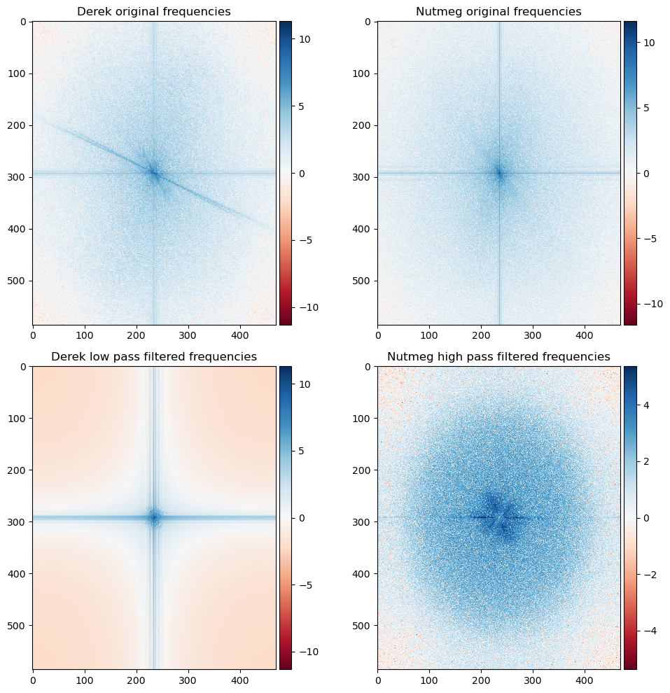
Now, we wish to analyze in the frequency domain what happend exactly in this process. This can be achieved by Fourier analysis. We first use scipy.fft.fft2 to transform the image into the frequency domain. Notice that fft2 outputs complex numbers and the zero frequency is located upper left corner [0,0] instead of the center of the image. We can use fftshift to move them back and use np.abs to get the magnitude of the component. I also used log-scale to better illustrate the weaker parts. We see in the case of a low-pass filter, only the frequencies around the two axes are preserved. This is the low frequency part of the signal. On the other hand, with the high frequency filter, we see a clear hollow spot at the origin, and the surroundings became significanly stronger. This is the high frequency part of the signal.

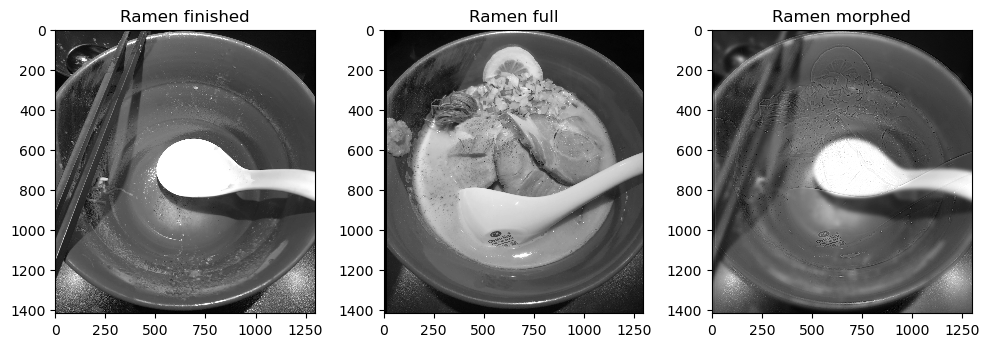
As a failing example, I show here a morphing between two bowls of ramen, one finished and one still full. However, as the background contains a spoon, the very strong contrast in the background survived through the low pass filter and result in a not so good outcome.

The following example is an successful one. It is morphing between airpods and Candace and Jeremy from phineas and ferb. Even though the black mics on airpods are a bit disturbing, the overall visual perception is pretty clean.

Part 2.3: Gaussian and Laplacian Stacks

To implament a Gaussian and Laplacian stack, we first take in an image, create a new image by convolving with a gaussian filter. Now, we add the convolved image to the Gaussian stack and the difference between the original and the convolved into the Laplacian stack. Next, the new image becomes the input and the process is repeated. An example of the stacks is shown below.

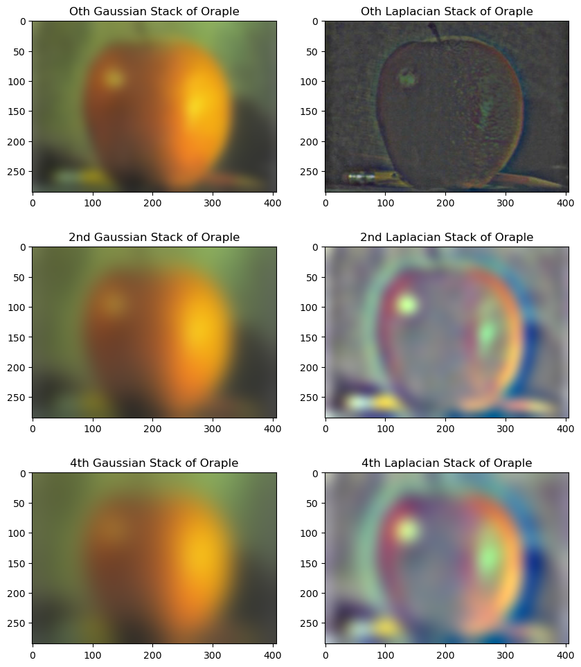
Here, to visualize the stacks, notice that laplacian stack becomes increasingly faint (low intensity), I renormalized it such that the maximum and minimum spans [0, 1]. Following the original paper, I visualized only the 0, 2, and 4th in the stack:

Part 2.4: Multiresolution Blending (a.k.a. the oraple!)

For sanity check, I visualized the oraple if we just stich them together. Not only the sharp edge is there the sizes also mismatch.

We then proceed to create the oraple. Note that the sum of the Laplacian stack and the last image in Gaussian stack will be the origin image. Therefore, we build a list, last image in Gaussian stack being the first, and the reversed Laplacian stack follows. In this way, it is sorted by the lowest frequency compoenets to the highest frequency components. Then, we use a window ratio (the proportion of the linear transition in the window) that gradually decays from 0.5 to 0.5 / 6 to force a seamless transition. The result looks like:

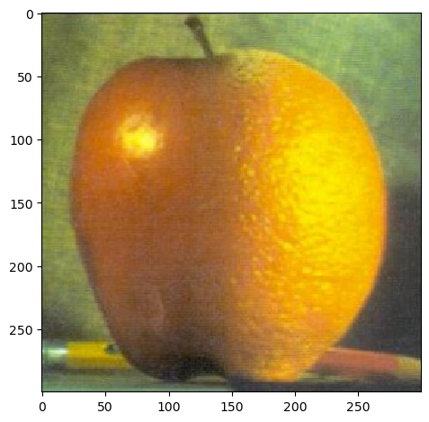
To illustrate the process, I blended a horse and a cow into what I called a “horow”:

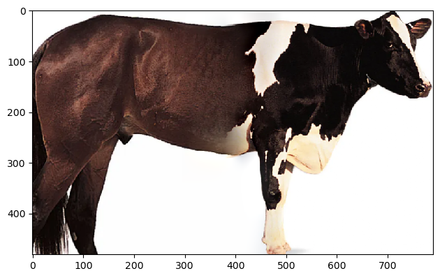
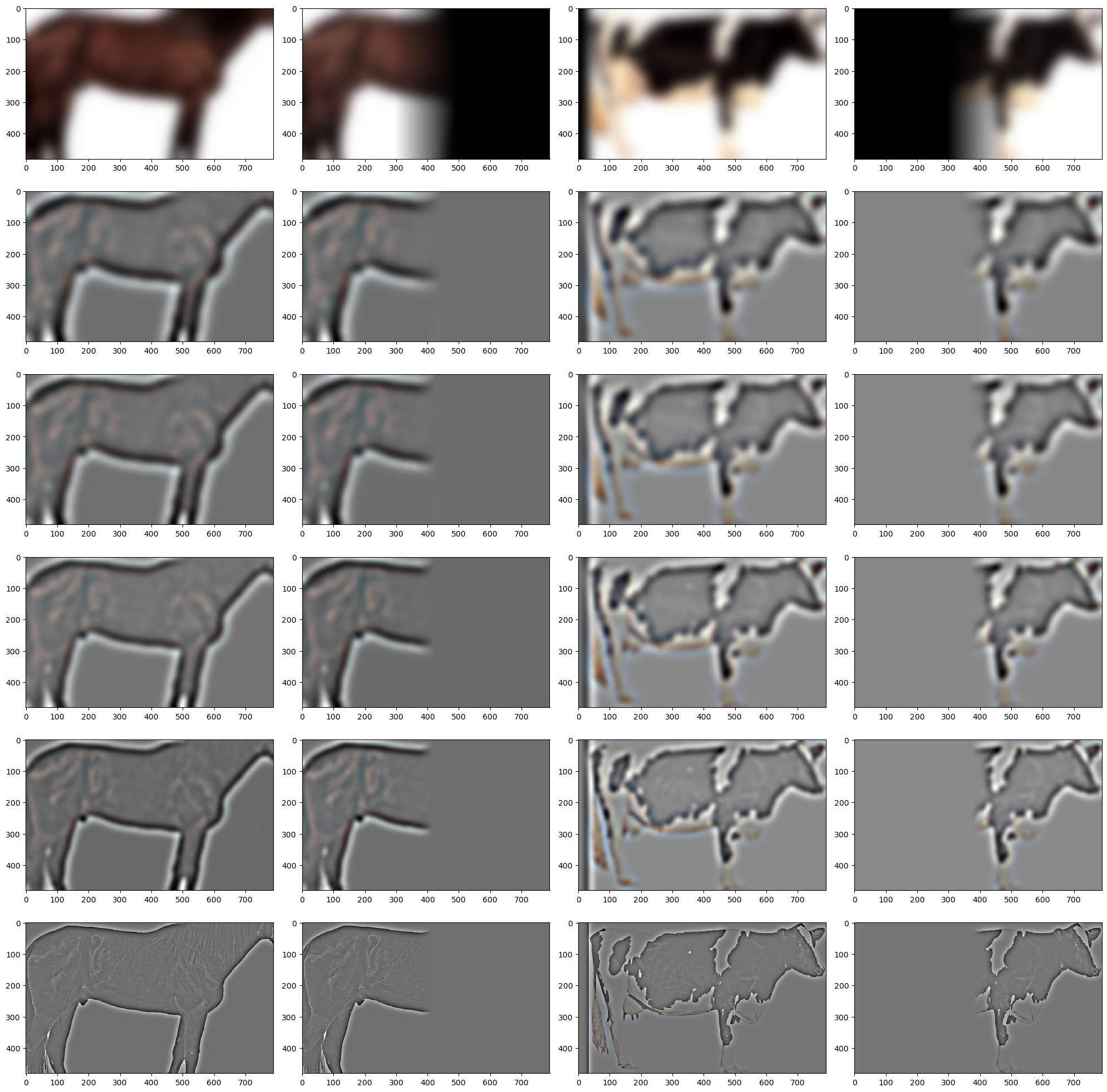
We can visualize the process by taking the images in the Laplacian and Gaussian stasks and the “masked” version of them (after applying the smooth transition). From the top we get the lowest frequency part (last of the Gaussian stack) to the highest frequency part (first in the Laplacian stack). The masked versions are shown to the right of the original in stack:

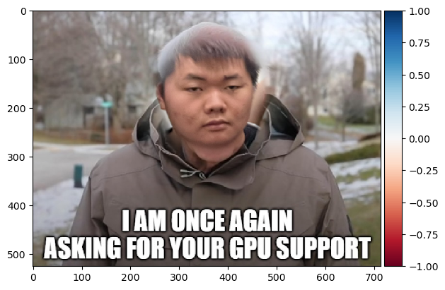
To be more flexible, I wrote a function that can generate circular masks. This allows one to choose a point in the image and replace it with a target in a specific radius. My first example will be merging Brandon, my friend at BAIR who has been crying for more GPUs for a long time, with a meme asking for more GPUs.

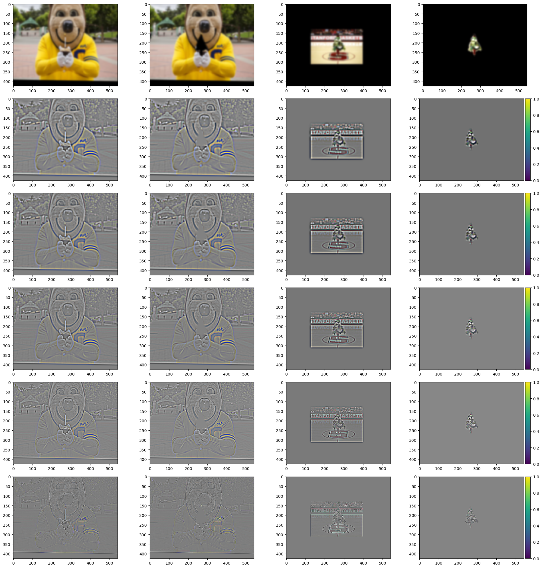
Finally, I am going to replace the cup cake and candle in Oski’s hand with the tree of the university across the bay.

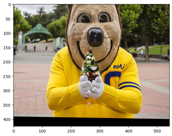
The process has also been visulized: