Introduction

In this project, I explored how to use a neural network to render novel views of a 3D object with the framework of neural radiance field (NeRF).

Part 1: Neural Field

Before tackling the harder task of 3D rendering, we can first take a detour to look at the 2D version of NeRF. the Neural Field. While NeRF fits a model to represent the function \(F: (x, y, z, \theta, \phi) \to (r, g, b, \sigma)\), the Neural Field fits a model to represent a 2D image as a function \(F: (x, y) \to (r, g, b)\).

Network Architecture

To build a Neural Field model, there are two key components: (1) featurization and (2) encoder.

Featurization is done by positional encoding, which maps a coordinate by

where \(x\in[0, 1]\) must be satisfied to ensure the uniquesness of the encoding. To generalize to higher-dimensional coordinantes, we simple concatenate the outputs of individually encoded results, which gives \(\mathbb R^{d(2L+1)}\) encoded vector.

The encoder is implemented by an MLP, with six configurable parameters: input dimension \(d_{i}\), hidden dimension \(d_{h}\), output dimension \(d_{o}\), number of layers \(n\), dropout \(p\), and activation \(\sigma(\cdot)\). The architecture is visualized as follows:

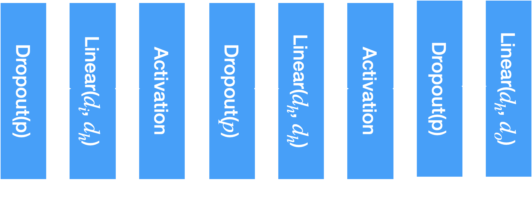
The block diagram of the MLP used in the project.

The encoder used for this part of the project has \(L=10\), \(d_{i}=42\), \(d_{h}=256\), \(d_{o}=3\), \(n=3\), \(p=0\), and activation is SiLU \(\sigma(x)=x\cdot\mathrm{sigmoid}(x)\). To make sure the output is in valid RGB range, the output is passed through a sigmoid to rescale it to \([0, 1]\) range.

Training Procedure

There are three major components of training the model: data loading, optimization, and evaluation.

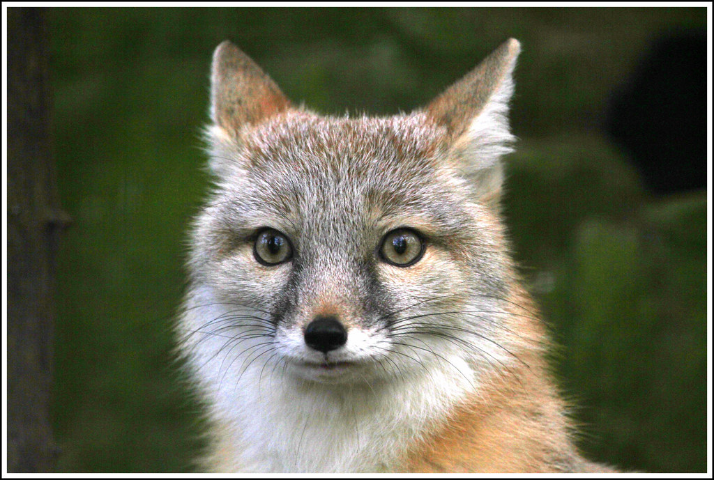
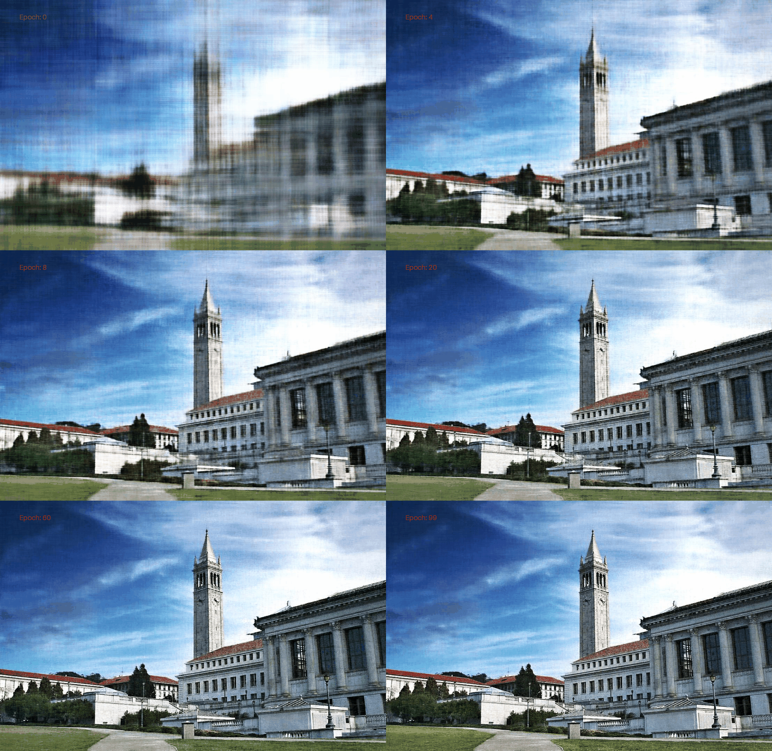
For data loading, instead of using the torch Dataset and DataLoader, I implemented a custom on-device data iterator. The advantage is that torch Dataloader is a multi-threaded CPU data loader. As our dataset is small (an image!) and batch size is large (~10K), it is more efficient to keep the entire dataset on the cuda device. The images used for training are shown below:

Fox

Memorial glade

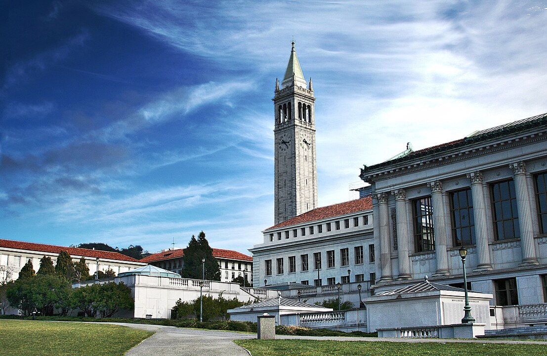
The images used to train the Neural Field model.

For optimization, I used the Adam optimizer with learning rate of 1e-2, weight decay of 0, and beta = [0.9, 0.999]. The batch size is set to 10000. A StepLR scheduler is also used with step size of 10 and gamma of 0.9. The model is trained for 100 epochs.

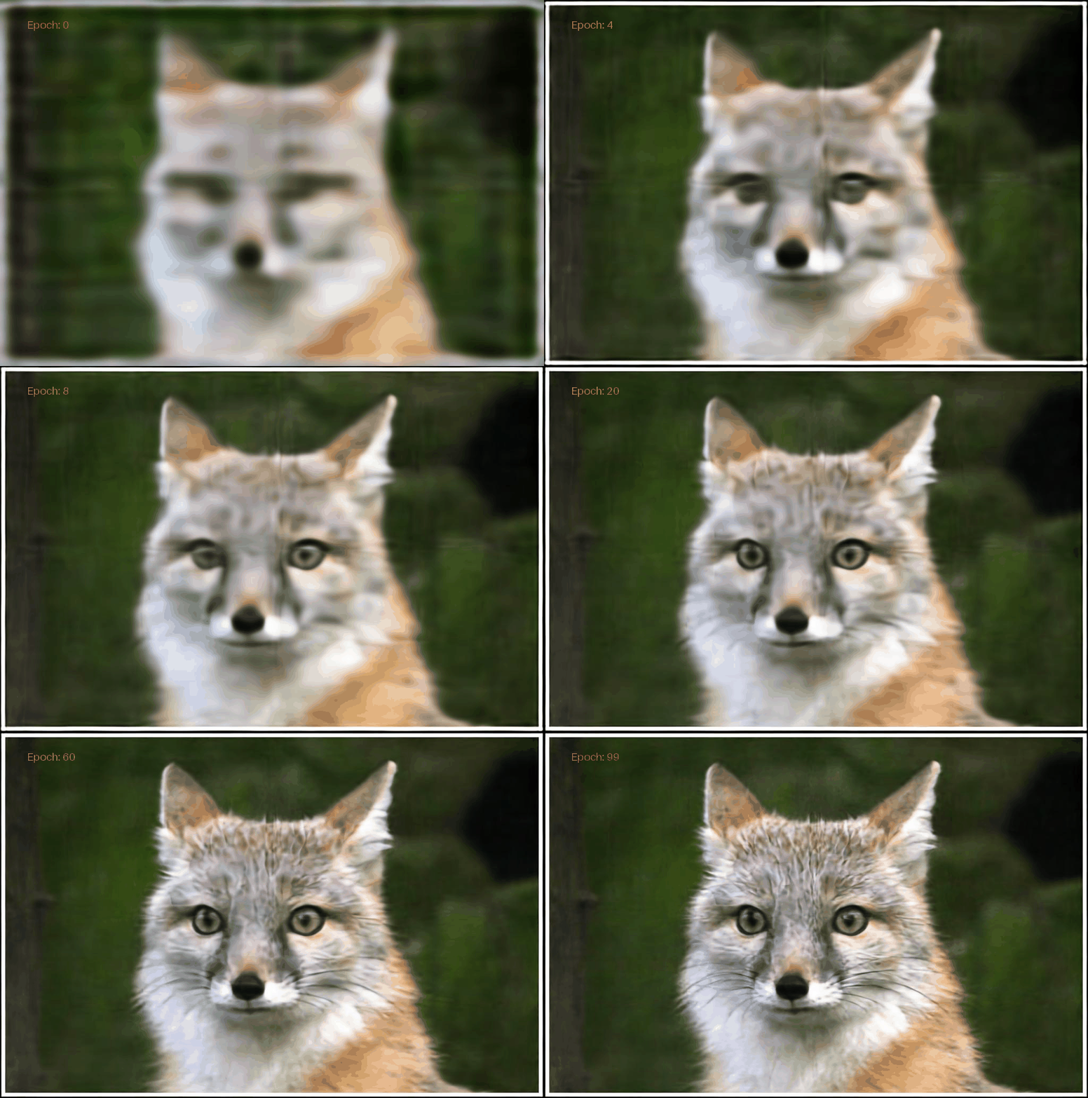
For evaluation, two metrics are employed: the MSE and PSNR. PSNR is defined as \(\mathrm{PSNR} = - 10\log_{10}(\mathrm{MSE})\). Notice that PSNR must be calculated after MSE aggregation per step since Jensen inequality implies PSNR is overestimated if calculated binned. The model checkpoint is saved along the training procedure and inferred to evaluate the model’s performance more intuitively.

Results and Ablations

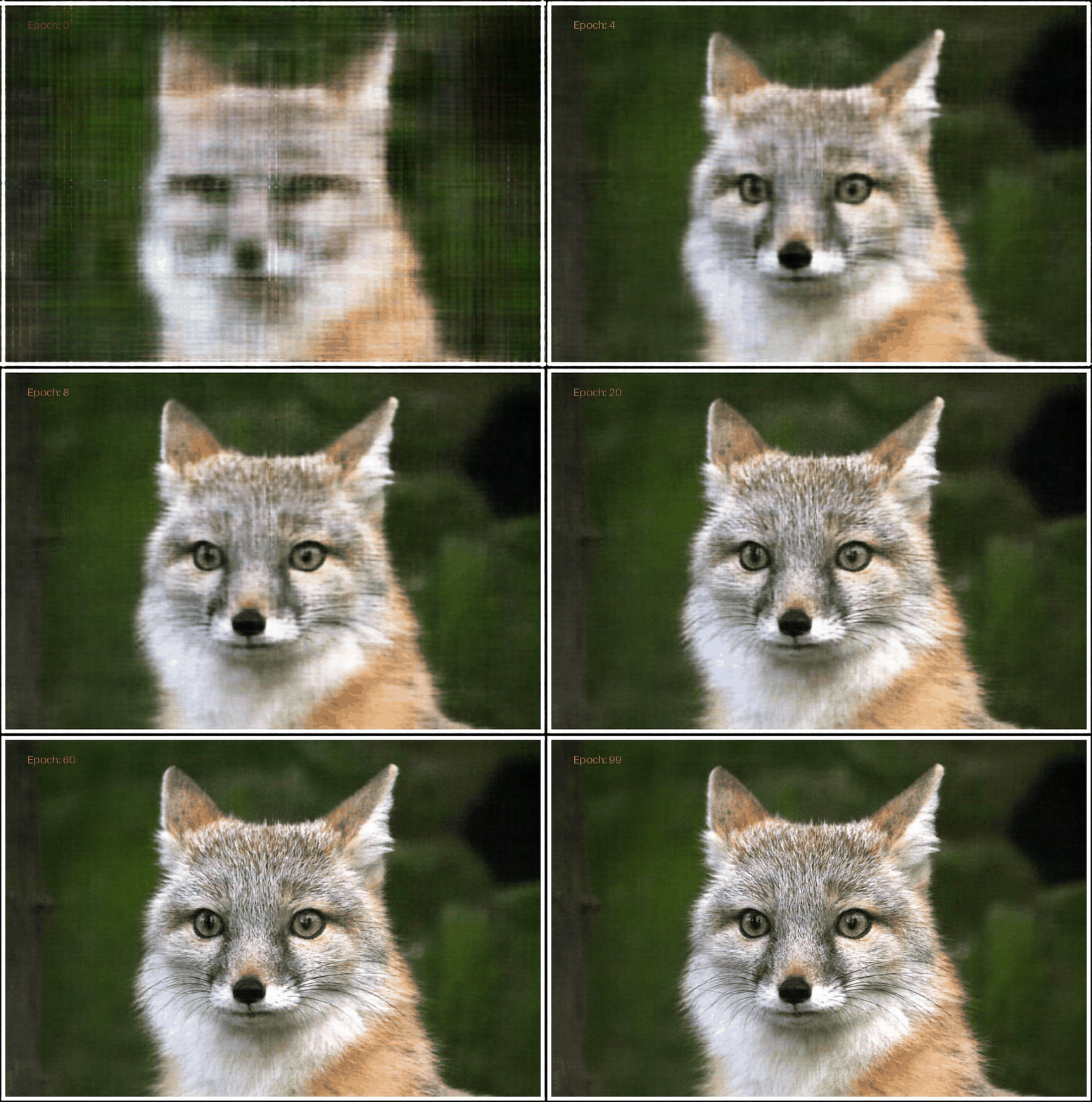
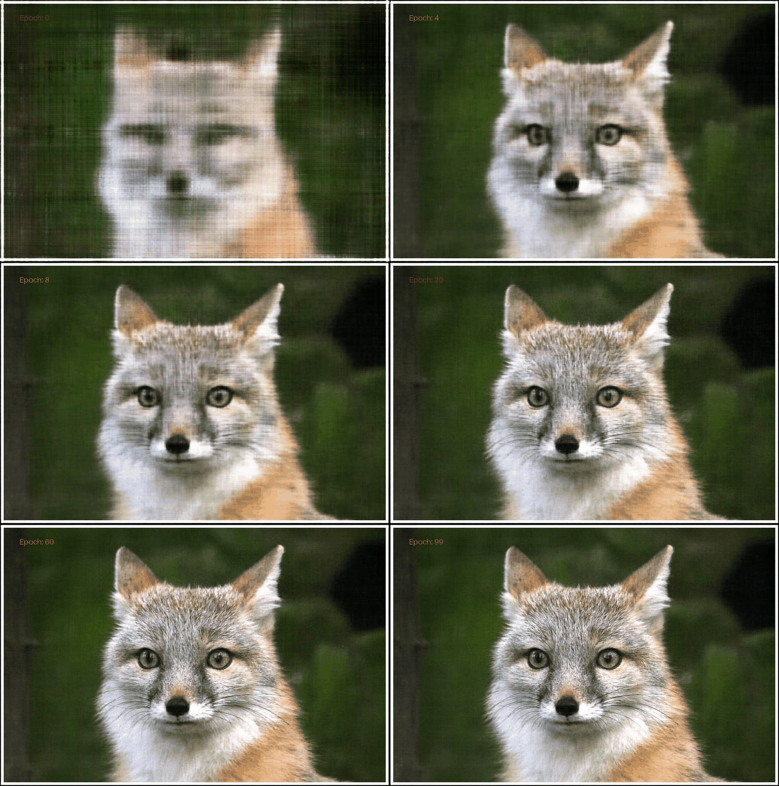
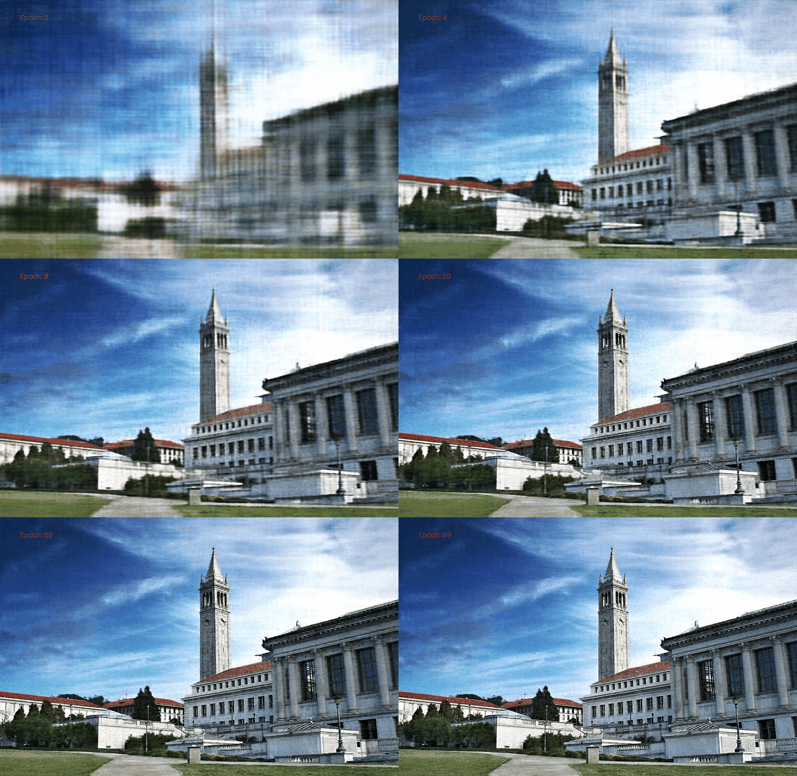
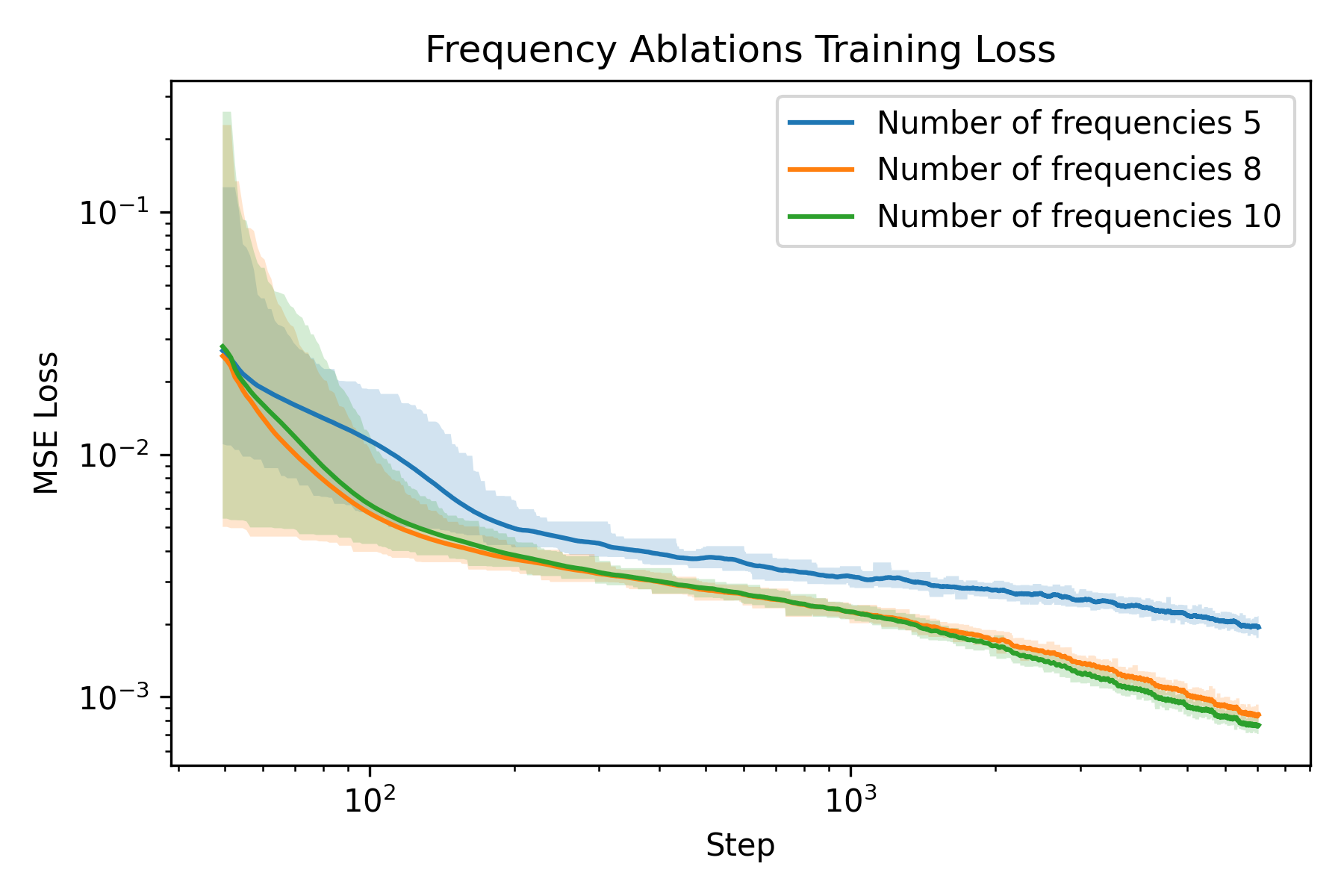
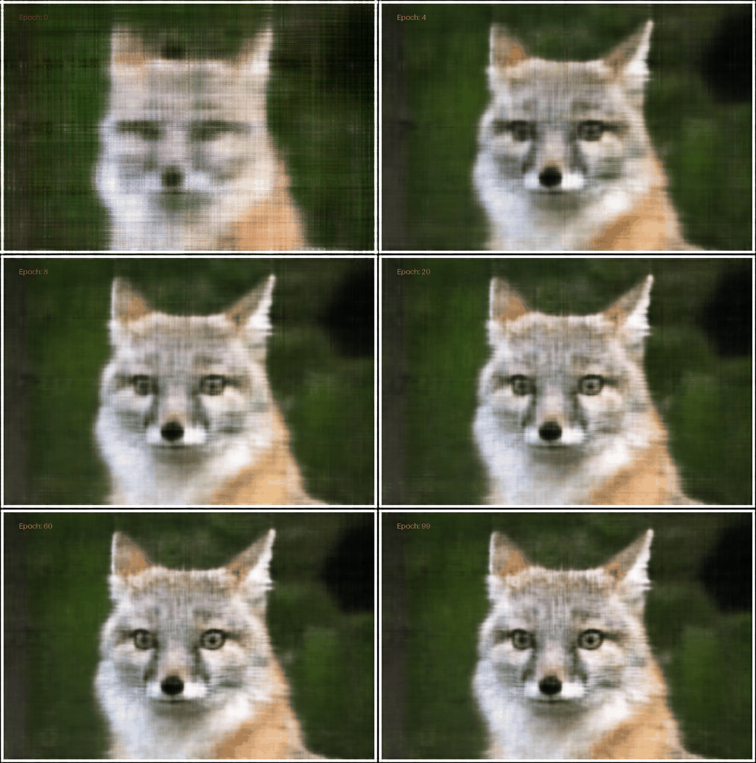
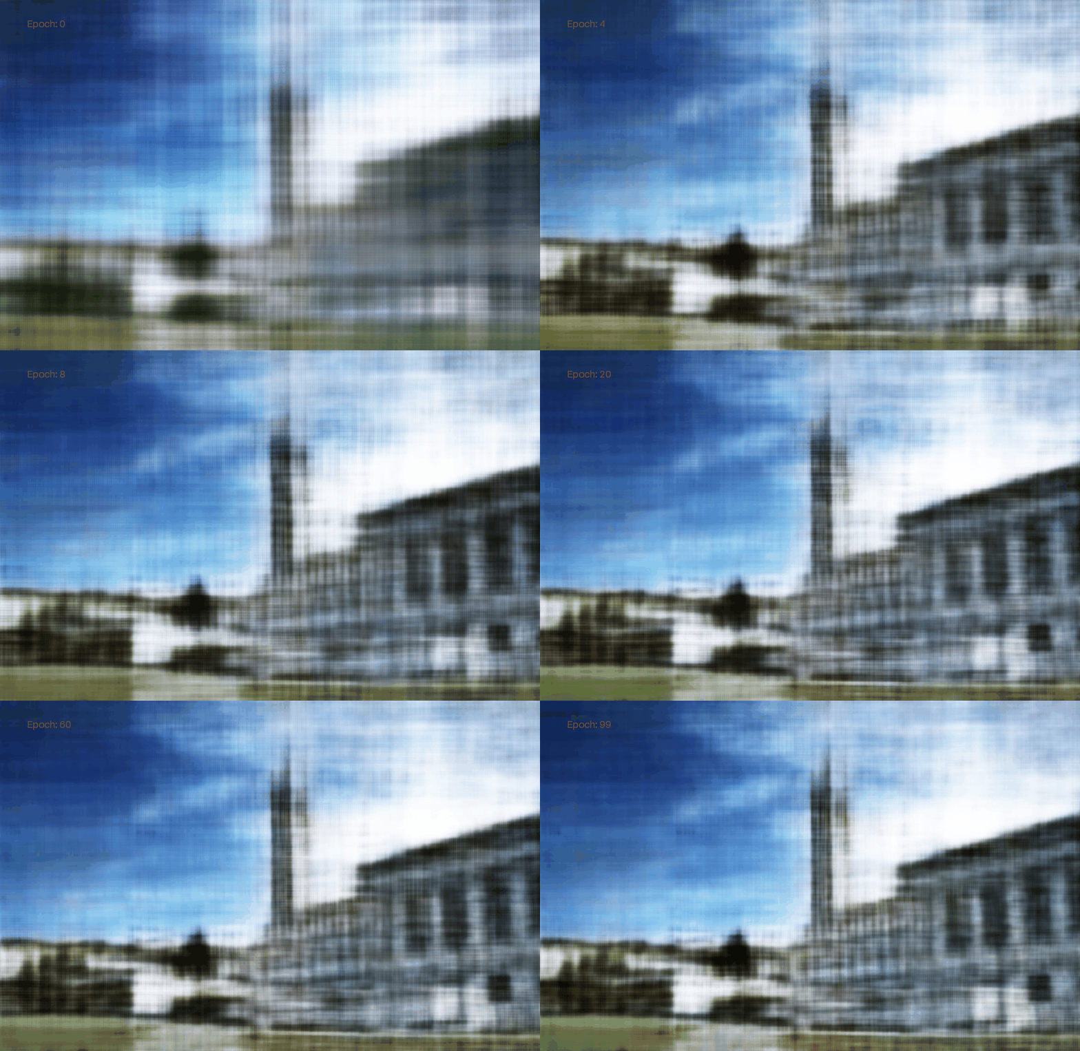
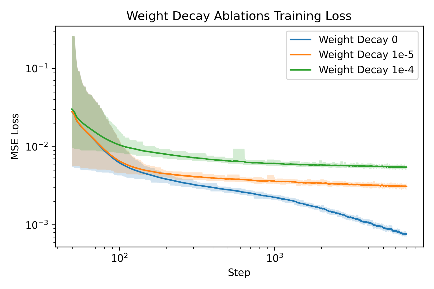
An ablation study is carried out to understand how to train a Neural Field better. The two parameters I chose to ablate on is the number of frequencies \(L\) and the weight decay of the Adam optimizer. The rationale behind the choice is that number of frequencies directly controls the resolution of our featurization, and weight decay regularizes the model to prevent overfitting, whereas overfitting is precisely what we want to achieve with the model.

$$L=5$$

$$L=8$$

$$L=10$$

Fox

Memorial glade

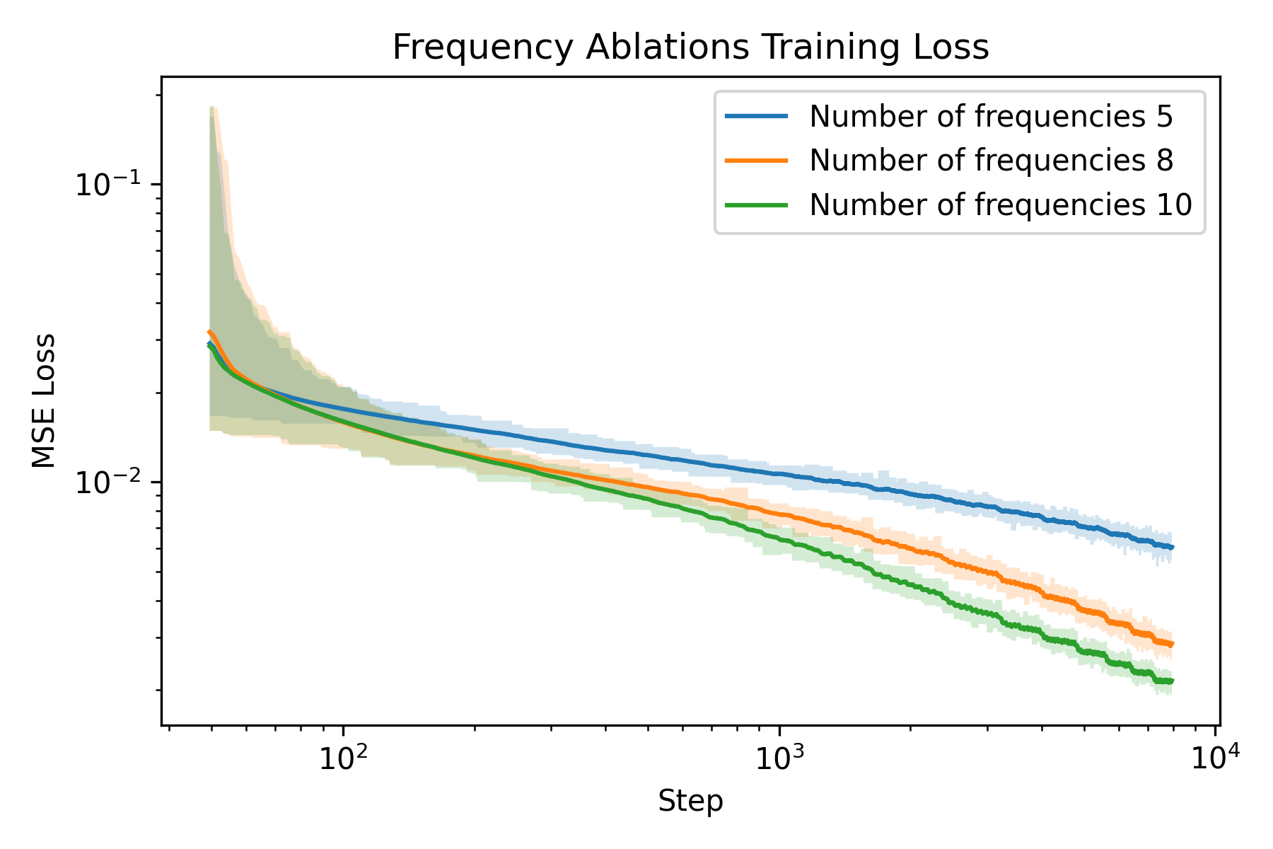
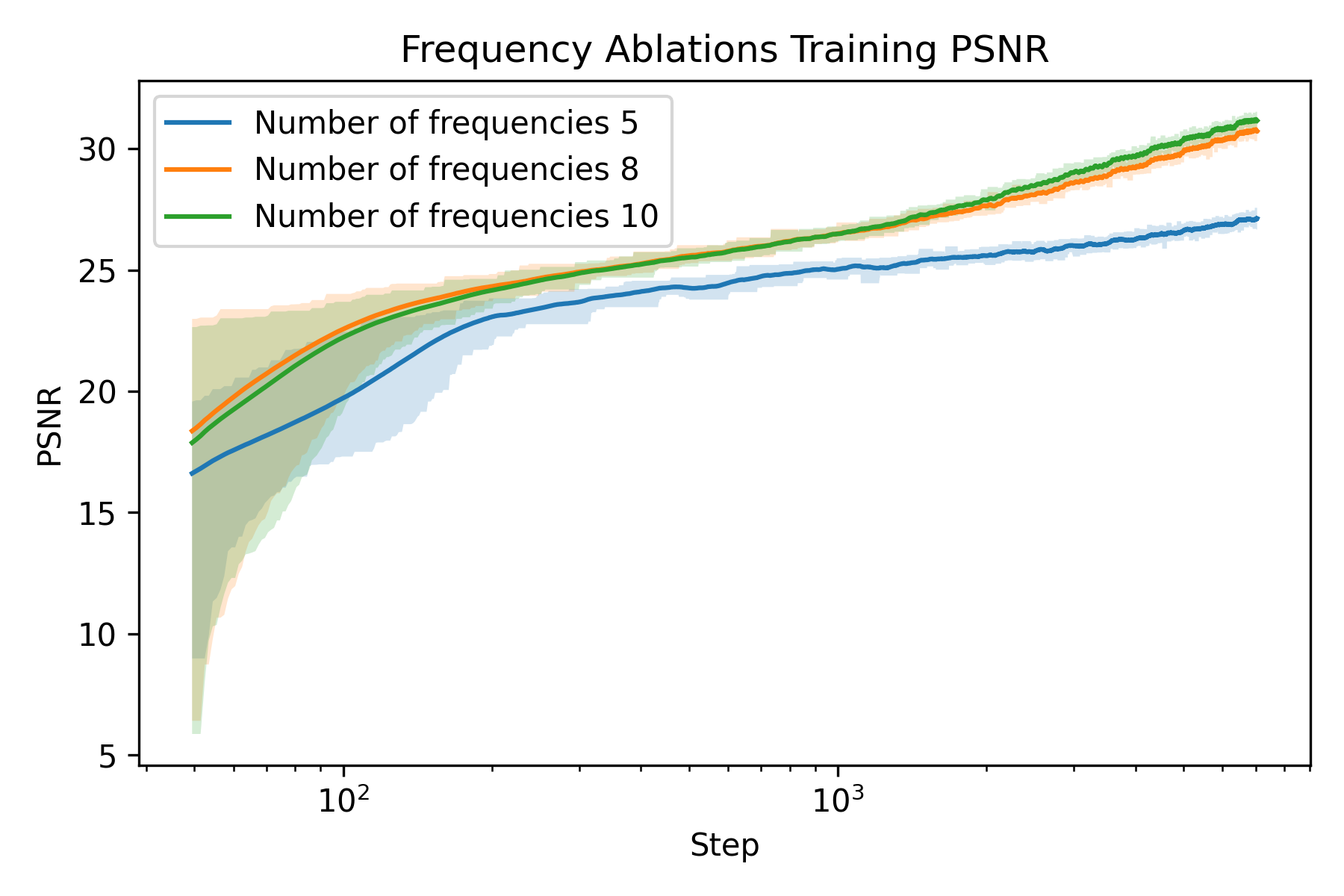
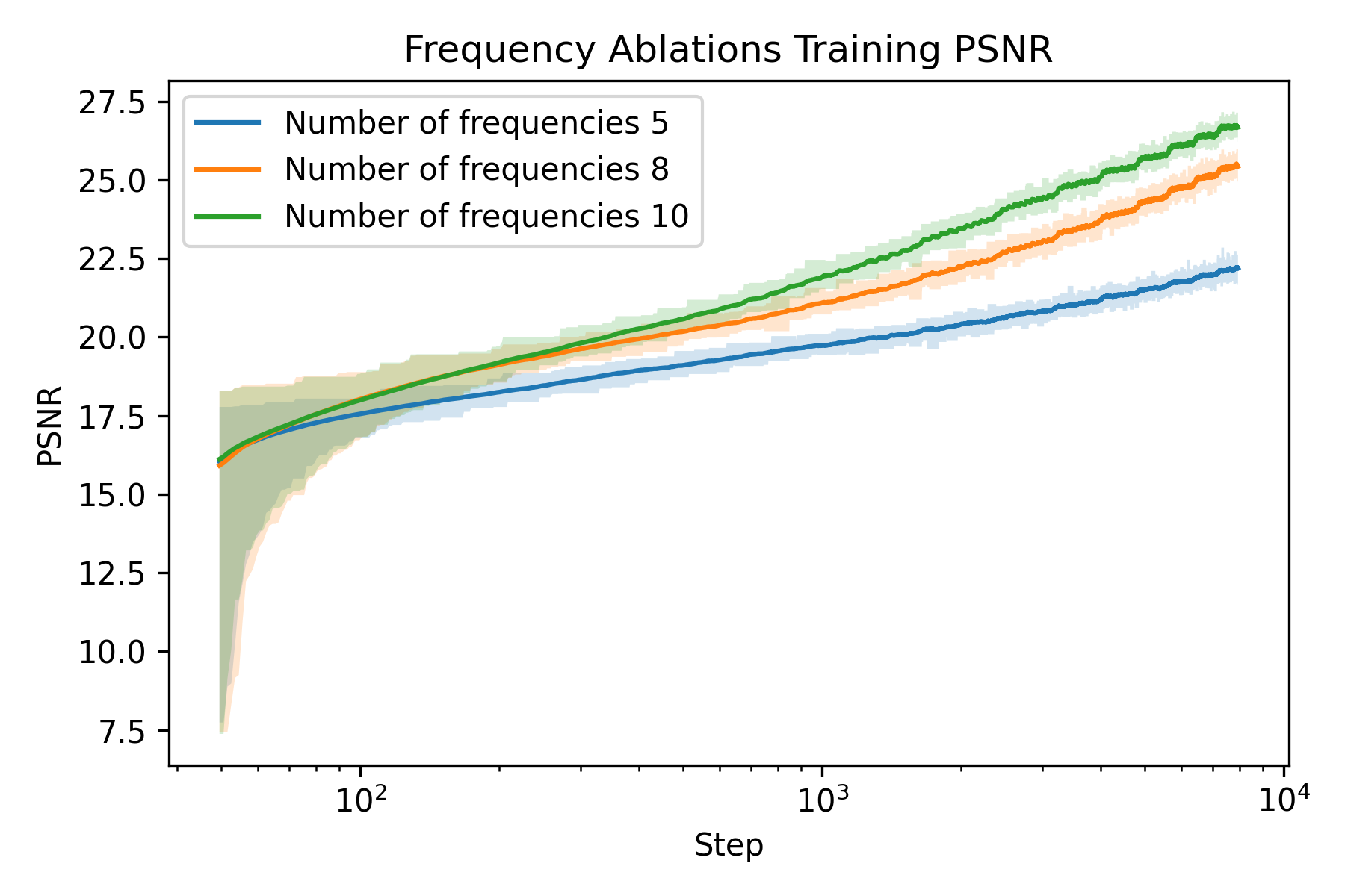
Ablation on frequency

We can see that at the beginning, the one with smaller number of frequencies are significantly worse than the ones with more frequencies. Moreover, we observe a larger gap in terms of PSNR for fox than glade. This is presumably due to more high frequency details in the fox image (hair). This verifies our hypothesis that more frequencies gives higher spatial resolution.

weight decay 0

weight decay 1e-5

weight decay 1e-4

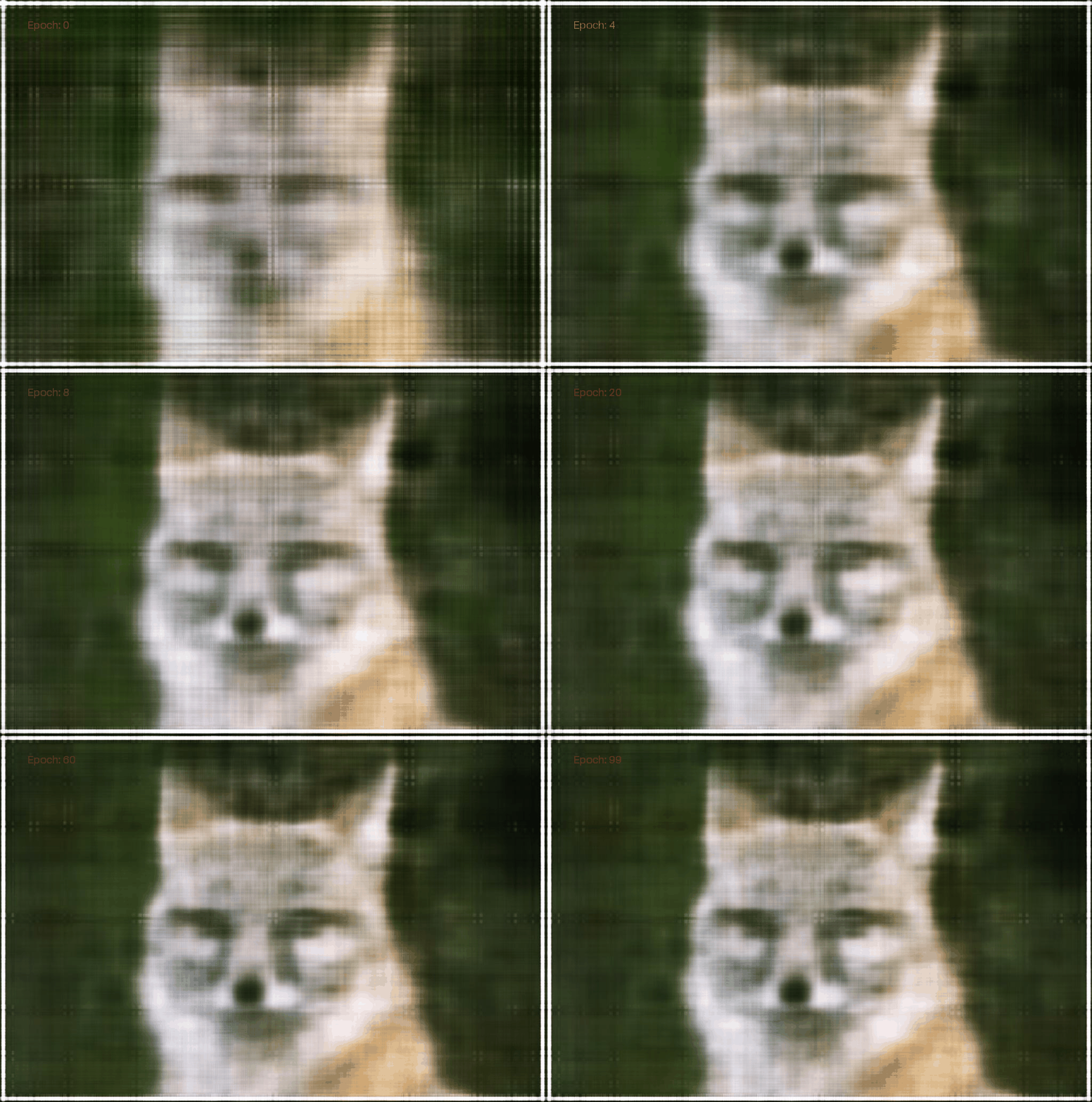
Fox

Memorial glade

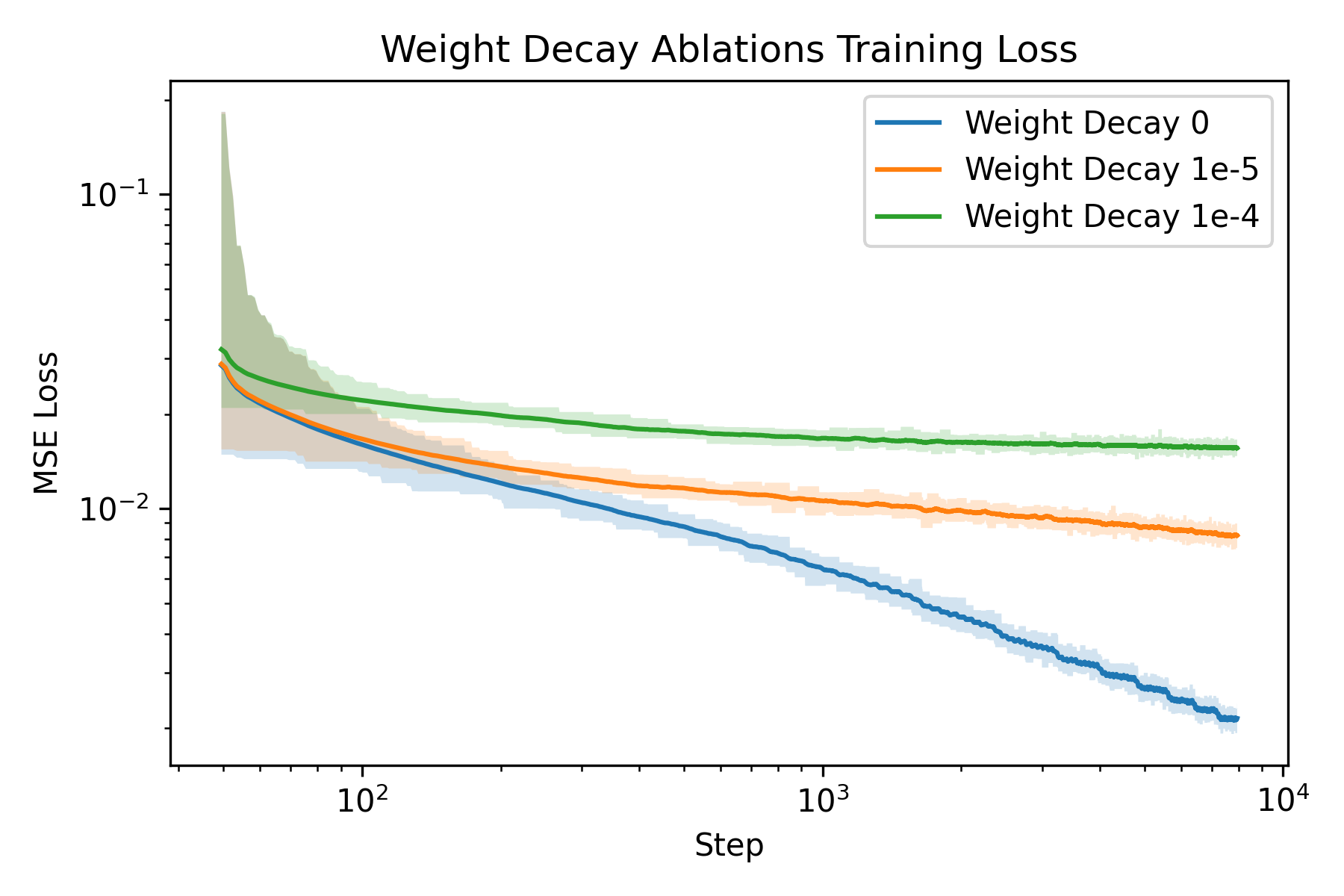
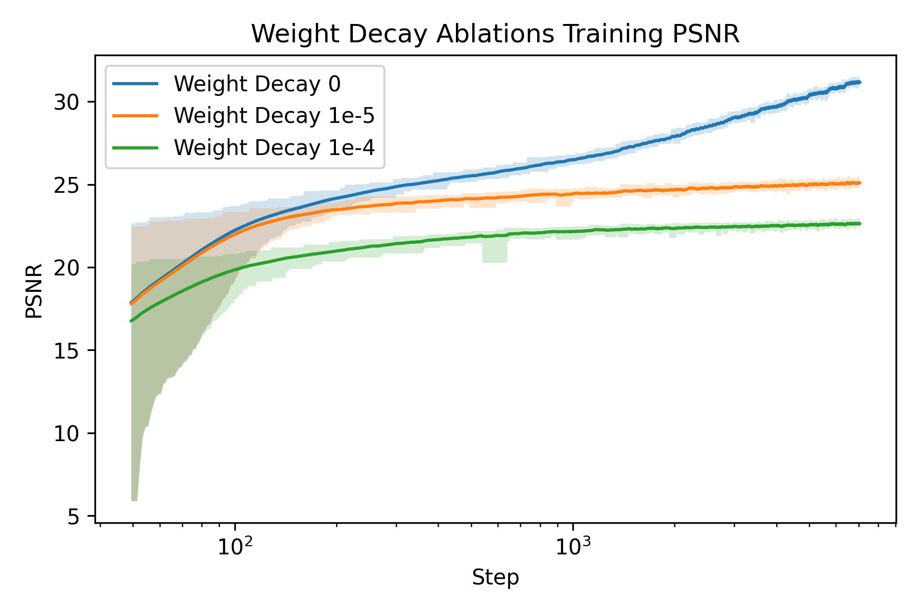
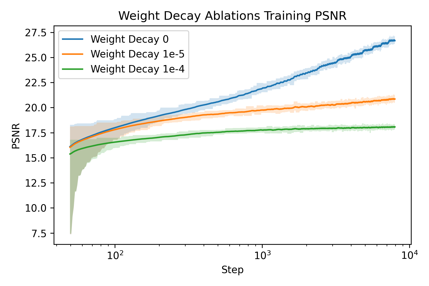
Ablation on weight decay

We can see that weight decay significantly impacted the model’s ability to “overfit” to the image as expected.

Part 2: Neural Radiance Field

Now we can proceed to use Neural Radiance Field (NeRF) to model 3D objects. As described in introduction, NeRF represents the scene with \(F: (x, y, z, \theta, \phi) \to (r, g, b, \sigma)\). However, we do not observe the world as a 3D volume. Instead, we see 2D renders of the scence. Therefore, we need to render the views during traning and inference time, which requires some theory to be worked out.

Theory

Our goal is to convert a pixel location \((u, v)\) into world coordinates \((x_w, y_w, z_w)\) along the ray. First, we define the pixel-to-ray transformation:

Therefore by inverting the intrinsic matrix \(K=\left[ \begin{matrix} f_x & 0 & o_x\\ 0 & f_y & o_y\\ 0 & 0 & 1 \end{matrix} \right]\), we arrive at the pixel-to-ray transformation:

where \(u\) and \(v\) are the center of the pixel, and \(s\) is the parameter that parametrize the ray. We can further transform the coordinantes in camera frame into world frame by using the equation:

Inverting it we get:

Notice that with \((x_c, y_c, z_c)=(0, 0, 0)\), we have \((x_w, y_w, z_w)=-\mathbf{R}_{3\times3}^{-1}\mathbf t\). Define the origin of the ray as:

Set \(s=1\) and apply the coordinate transformation, we can get a point along the ray direction \(\mathbf{X}_w\). Then we can define the ray direction vector by:

Using these two vectors, we can efficiently sample points along the ray by \(\mathbf{X}_t = \mathbf{R}_o + t\mathbf{R}_d\)

Suppose that we know the radiance field along the ray. How can we render the pixel values correpsonding to the ray? This requires volume rendering, which is defined as follows:

where \(T(t):=e^{-\int_{t_i}^t\sigma(\mathbf{r}(t'))\mathrm d t'}\). We can discretize the integral and get an estimator:

where \(T_i = e^{-\sum_{j=1}^{i-1}\sigma_i \delta_t}\).

Network Architecture

Similar to Neural Field, the two main components are still featurization and encoder. As the input is now a five-tuple of \((x, y, z, \theta, \phi)\), we need to rethink the way to featurize it. \((\theta, \phi)\) can be equivalently represented by a three-unit-vector \(\mathbf{R}_d\), which is the ray direction. Therefore, we use two positional encoders to encode them. Notice that \((\theta, \phi)\) does not require a high spatial resolution as it always lies on an unit sphere. Therefore we use \(L=10\) for \((x, y, z)\) and \(L=4\) for ray directions.

Another important design choice is to make \(\sigma\) independent of ray direction. This essentially requires transparency to be isotropy. This holds true for most materials with very few exceptions, and LEGO is certainly not one of them. The final architecture design is showned below:

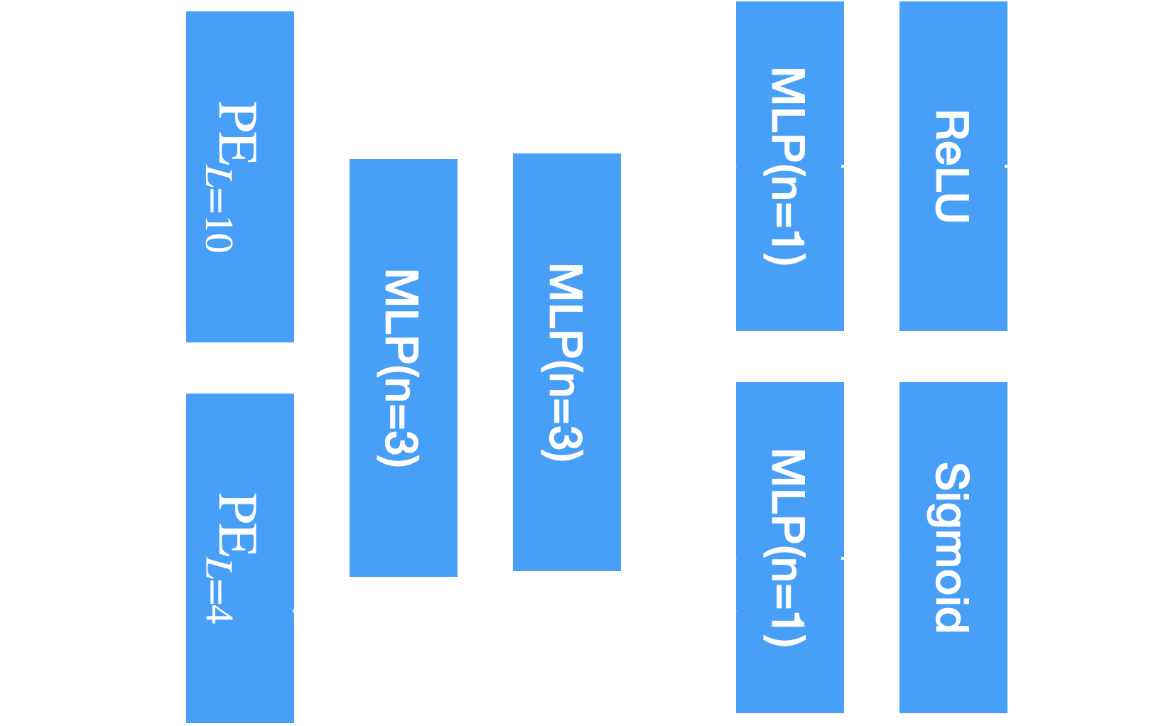
The block diagram of the network used for NeRF

The MLP has hidden dimensions of \(256\) and the inputs are concateneted when there are multiple inputs to the MLP. The first two blocks have \(3\) layers, and the output blocks have \(1\) layer (\(L\)-layered MLP has \(L+1\) linear layers).

Training Procedure

For data loading, we use the theory developed in the theory section and preprocess rays into the vectors to represent them. Given 100 images with \(200\times200\) resolution, there are 4,000,000 rays in total. Though it seems to be a large number, it can fit into the cuda device and for the same reason it will be more efficient to store them on-device. For each batch, we sample points along ray by creating a evenly spaced sequence of \(t\) from \(2.0\) to \(6.0\) with torch.linspace(2.0, 6.0, 64). Gaussian noise with \(\sigma=0.01\) is added to the sampled \(t\). The sampled points and the correpsonding pixel values are returned. An example of 100 rays sampled is shown below:

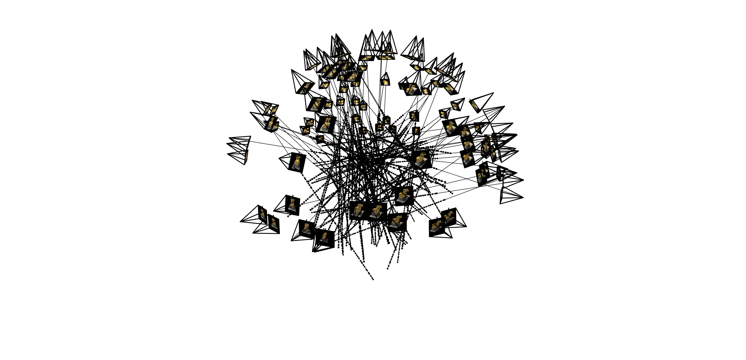
100 random rays and the sampled points.

For each pair of ray and pixel values, we evaluate the model on these points and use volume render equations to get the predicted pixel values and train with MSE loss. For the default configuation (from spec), the optimizer is Adam with a learning rate of 5e-4 and no weight decay. No learning rate scheduler is used, and the batch size is 10000. The model is trained for 100 epochs, which took about 1.5 hours on one RTX 3090. As one of the Bells & Whistles (PSNR > 30), I also experiemented with advance learning rate schedule. This includes starting with a higher learninng rate of 8e-4 and using a CosineAnnelaingLR scheduler with eta_min of 1e-5. The parameters are not tuned, and the rationale behind the choice is to cover a wider range of learning rate to encourage learning at different scales. This model is labeled “advance” in the results section.

To evaluate the model, validation loss and PSNR are reported. I also rendered validation views to provide more intuitive assessment to the model’s performance.

Results

Firstly, the training and validation curves of NeRF is shown as follows:

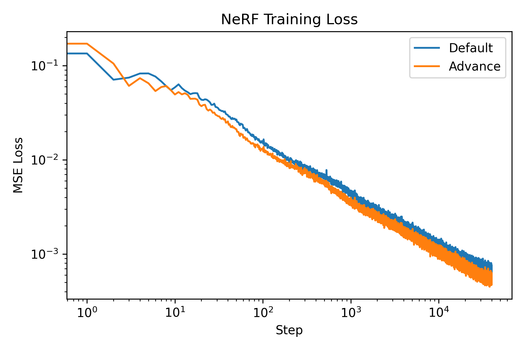
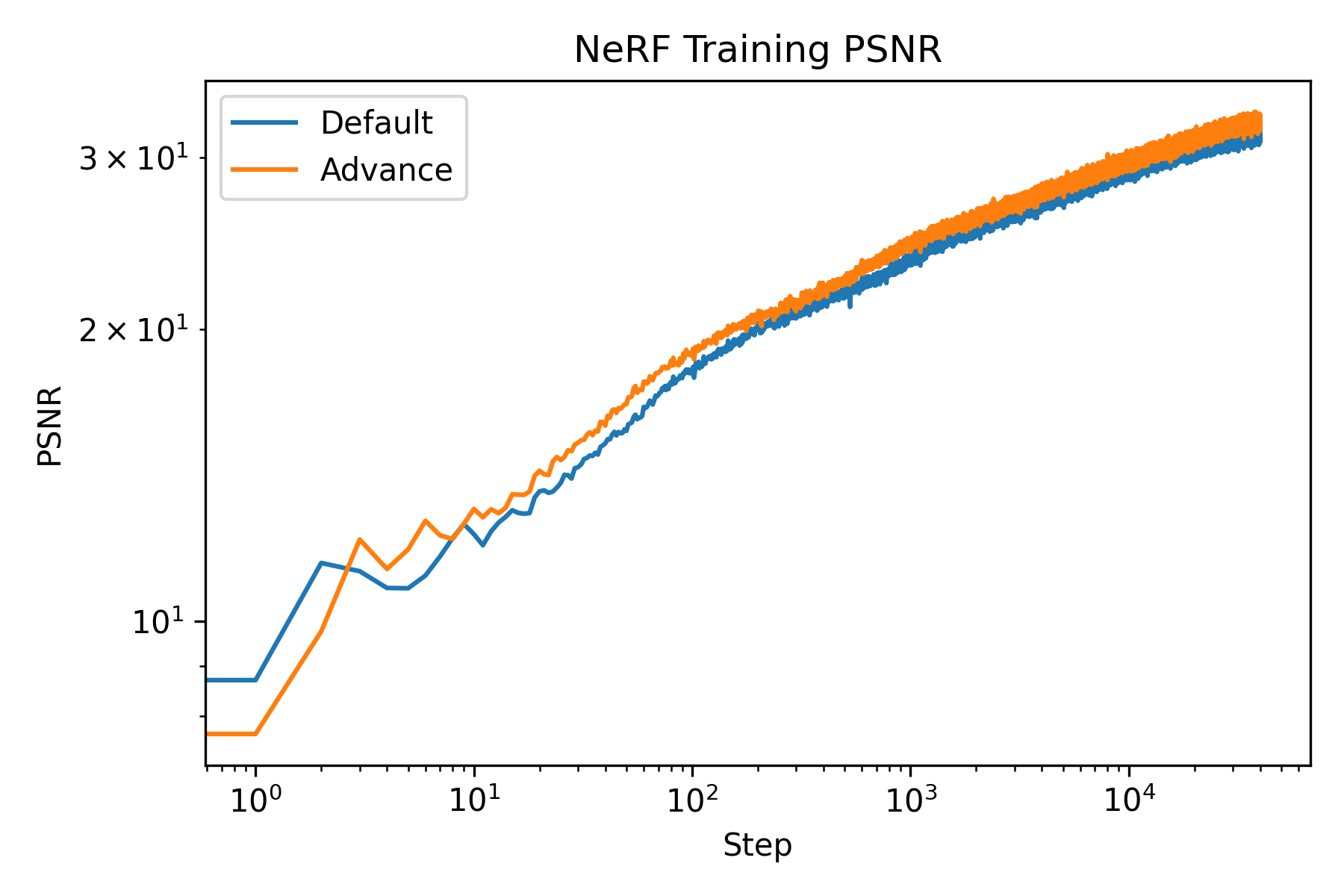
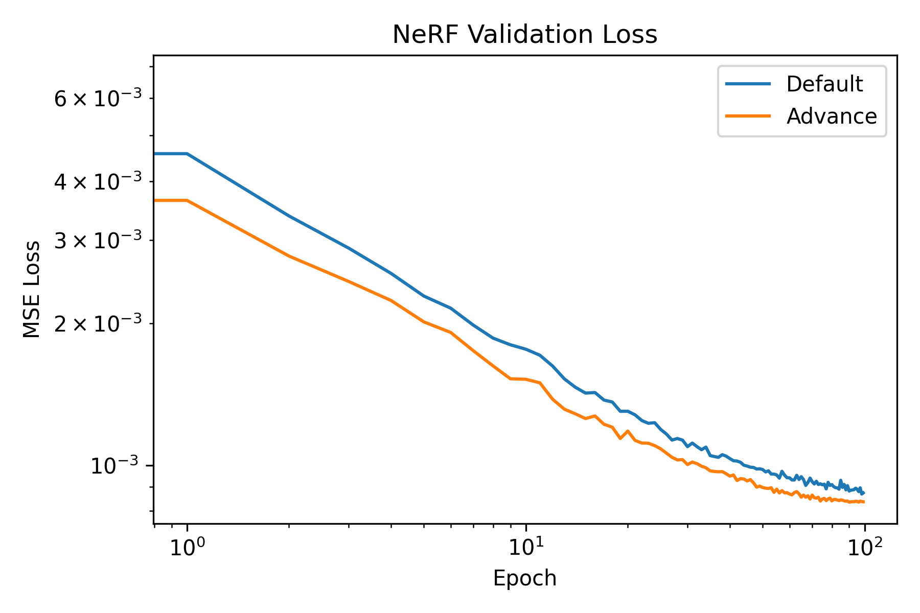
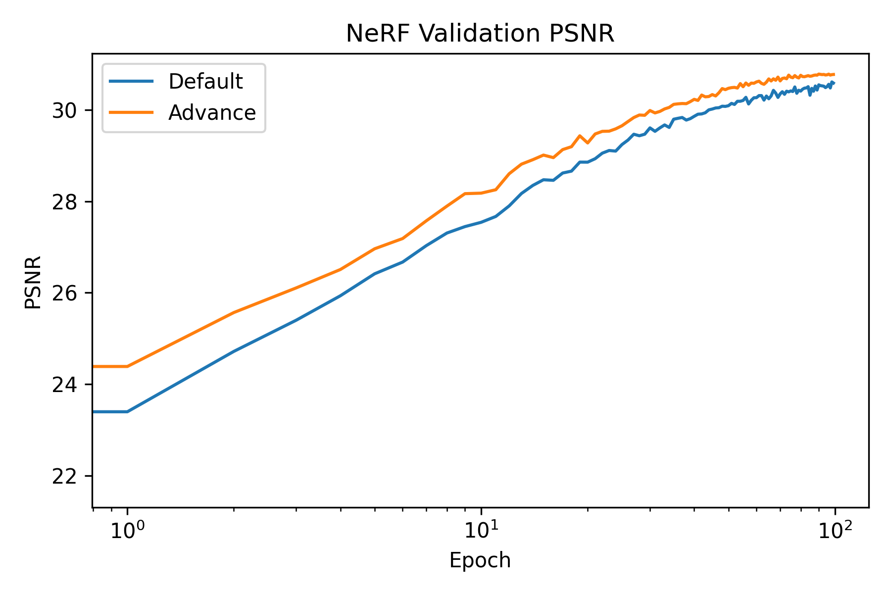
The training and validation curves of NeRF.

We see that both model achieved high PSNR. Moreover, the advance one achived a PSNR higher than 30. To visually assess the model’s performance, we can visualize the validation views throughout the training process.

Epoch 0: Default

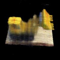
Epoch 0: Advance

Epoch 1: Default

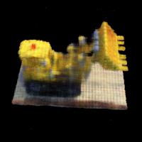
Epoch 1: Advance

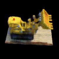
Epoch 2: Default

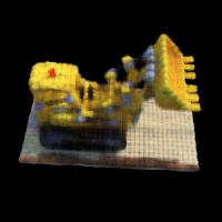
Epoch 2: Advance

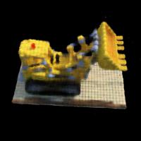
Epoch 3: Default

Epoch 3: Advance

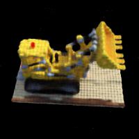
Epoch 4: Default

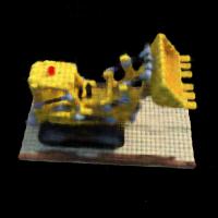
Epoch 4: Advance

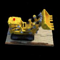
Epoch 10: Default

Epoch 10: Advance

Epoch 50: Default

Epoch 50: Advance

Epoch 99: Default

Epoch 99: Advance

The difference between the two are visually marginal.

Finally, we can render novel views with the test set:

Default

Advance

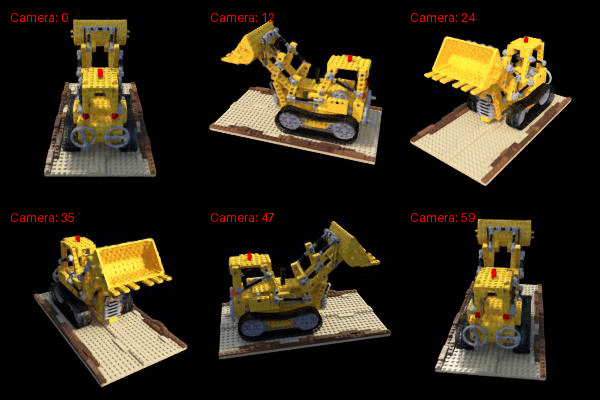
Rendering results on test set

We see both model generates good 3D views.

Rendering with Background colors

Finally, we can try changing the background colors. Notice that in the volume rendering equation, while a ray with many points of high \(\sigma_i\) would have very small \(T_i\), the probability of the ray terminating, at the end, it is generally not guaranteed that this will always be the case. If we think of volume rendering as an weighted average, then with \(T_N\neq 0\) we are essentially getting a point with weight \(1 - T_N\) with RGB all being zero. This is the black background we are getting. We can render the background with different color by adding \((1-T_N)*\mathbf{c}\) to the volume rendering process. This can be easily implemented by appending torch.inf to the \(sigma\) array and the desired background color to the \(rgb\) array. An example of rendering with background is shown below:

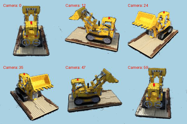
Rendering with another background color

We see that there are some black noise in the background. This is due to the fact that if the model predicts black with high sigma it can still accurately describe the training image. This can be resolved by using PNG images with proper alpha channels.